1.1.9.4. 2D Finite Volume Method: Non-Cartesian Grids
1.1.9.4.1. Summary
The cross product is used to compute the volume
The midpoint rule is used to compute the flow quantity and the source term
The FVM with the cell-centred or cell-vertex formulation can be used to compute the fluxes
If the FVM is applied on a Cartesian grid (every angle is a right angle), the FD formulas are recovered
1.1.9.4.2. Non-Cartesian Grid
Non-Cartesian, although shown as Cartesian, but we will not assume we know the volume of the cell ABCD
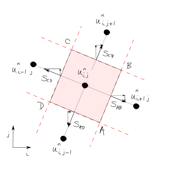
For cell ABCD:
where: \(f\) and \(g\) are the Cartesian components of the flux vector \(\mathbf{F}\)
The sign in the flux appears due to the surface vector, e.g for Side AB:
1.1.9.4.3. Evaluation of the Flow Quantity Terms
Can use midpoint rule which approximates a volume integral by the product of the centre value and the CV:
1.1.9.4.4. Evaluation of the Source Terms
Can use midpoint rule which approximates a volume integral by the product of the centre value and the CV:
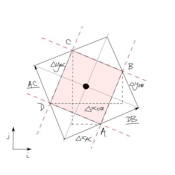
1.1.9.4.5. Evaluation of the Volumes
The vector product is the area of a parallelogram
Take the absolute value to ensure the value is positive (\(\Delta x\) and \(\Delta y\) can be negative)
The area we are looking for (the quadrilateral) is half the area of the parallelogram:
1.1.9.4.6. Evaluation of the Fluxes
The evaluation of fluxes determines the difference between a variety of schemes, e.g. cell vertex or cell centered
It depends on the location of the flow variables w.r.t. the mesh and selected scheme
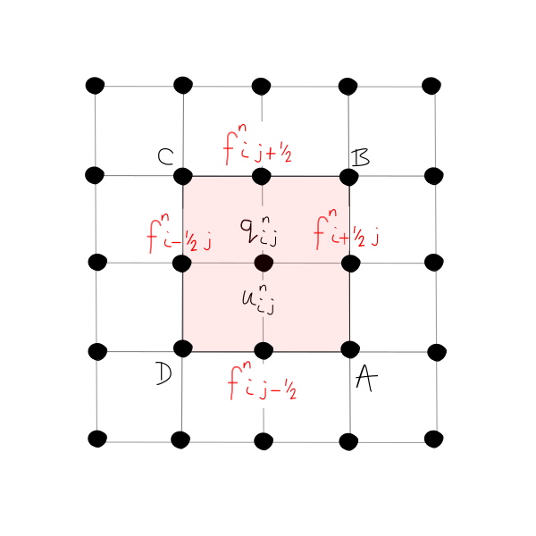
1.1.9.4.6.1. Central Scheme and Cell Centered FVM
We know the values at the black dots, we don’t know the values in red

Option 1: Average of fluxes perpendicular to face - e.g. midpoint rule
Take the average flux:
where \(f_{i,j} = f(u_{i,j})\)
Flux of the average flow quantity:
(not the same, because f is generally non-linear)
Can also use Upwind, Linear Interpolation, QUICK and Higher Order Schemes for midpoint rule
Option 2: Average of fluxes parallel to face A and B - e.g. trapezoid rule
Evaluate flow quantity in A and B (at the corner A)
Or average the fluxes:
(more flux evaluations - could be expensive computationally)
Can also use Simpson’s Rule, cubic polynomials for this type of rule
1.1.9.4.6.2. Central scheme and Cell Vertex FVM
We know the values at the black dots, we don’t know the values in red - remember flux is not at a point, it’s through a face by integration.
Option 1 - fluxes perpendicular to face:
Option 2 - fluxes parallel to face:
The last one corresponds to trapezoidal rule for the integral:
Summing over the sides ABCD:

Use trapezium rule: half the sum of the parallel sides times the distance between them:
1.1.9.4.7. 2D Example - FVM Reduces to FD
This is a generic example - we could use cell centered or cell vertex here (but just showing cell centered):

For cell ABCD:
Volume:
\(\Omega_{i,j} = \Delta x \Delta y\)
Surfaces:
\(\Delta y_{AB}\) = \(\Delta y\) \(\quad\) \(\Delta x_{AB}\) = \(0\) \(\quad\) \(\Delta y_{BC}\) = \(0\) \(\quad\) \(\Delta x_{BC}\) = \(\Delta x\) \(\quad\) \(\Delta y_{CD}\) = \(\Delta y\) \(\quad\) \(\Delta x_{CD}\) = \(0\) \(\quad\) \(\Delta y_{DA}\) = \(0\) \(\quad\) \(\Delta x_{DA}\) = \(\Delta x\)
Fluxes:
\(f_{AB}\) = \(f_{i+1/2,j}\) \(\quad\) \(g_{AB}\) = \(0\) \(\quad\) \(f_{BC}\) = \(0\) \(\quad\) \(g_{BC}\) = \(g_{i,j+1/2}\) \(\quad\) \(f_{CD}\) = \(-f_{i-1/2,j}\) \(\quad\) \(g_{CD}\) = \(0\) \(\quad\) \(f_{DA}\) = \(0\) \(\quad\) \(g_{DA}\) = \(-g_{i,j-1/2}\)
Hence:
Dividing by the volume we have recovered the finite difference formula:
Note: \(f_{i,j}\) and \(g_{i,j}\) do not appear, hence odd-even decoupling can occur