1.1.9.5.1. Summary of Previous Work¶

The Finite Volume Method is the most widely used method in CFD because it is applicable for any geometry and is therefore useful in engineering problems.

Fluxes are calculated at the faces of the control volumes. The way the fluxes are calculated determines which scheme is used. Previously we used a central scheme for these fluxes (the average of the fluxes at the points on each side of the face)

1.1.9.5.2. Two Options for Central Scheme¶

Choices for fluxes were:

• Central scheme with cell centered grid

• Central scheme with cell vertex grid

1.1.9.5.3. Cartesian Grid¶

Previously obtained this by dividing by volume:

This result is identical to the central difference formula, but this is only when we specify a Cartesian Mesh.

Still need to choose how to calculate the fluxes

1.1.9.5.4. Flux Calculation¶

1.1.9.5.4.2. Central Scheme: Cell Vertex¶

Alternative:

\[f_{AB} = {1 \over 2}(f_A + f_B)\]

Where:

\[f_A = {1 \over 4}(f_{i,j} + f_{i+1,j} + f_{i+1,j-1} + f_{i,j-1})\]

We obtain:

\[\begin{split}{\partial \over \partial t} u_{i,j} + {1 \over 4} \left[ {2({f_{i+1,j} - f_{i-1,j}}) \over {2 \Delta x}} + {({f_{i+1,j+1} - f_{i-1,j+1}}) \over {2 \Delta x}} + {({f_{i+1,j-1} - f_{i-1,j-1}}) \over {2 \Delta x}} \right] + \\ {1 \over 4} \left[ {2({g_{i,j+1} - g_{i,j-1}}) \over {2 \Delta y}} + {({g_{i+1,j+1} - g_{i+1,j-1}}) \over {2 \Delta y}} + {({g_{i-1,j+1} - g_{i-1,j-1}}) \over {2 \Delta y}} \right] = q_{i,j}\end{split}\]

Central FVM leads to 2nd order accuracy in space (although this depends on the mesh quality)

Problem: Central Scheme is unable to identify the direction of the flow

Solution: For convection dominated flows we need to use upwind, because it is then biased in the direction of the flow

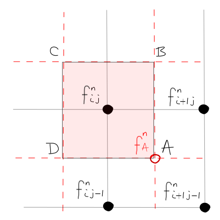
1.1.9.5.4.3. Upwind Scheme: Cell Centered¶

Evaluate fluxes in function of the propagation direction

Find the propagation direction by:

\[\mathbf{A}(U) = {{\partial \mathbf{F}} \over {\partial U}} = a(U) \mathbf{i} + b(U) \mathbf{j}\]

with \(a(U) = {{\partial f} / {\partial u}}\), \(b(U) = {{\partial g} / {\partial u}}\)

The Jacobian represents the direction of propagation - e.g. the simplest possible Jacobian is the wave speed for 1D linear convection - positive A is left to right, negative A is right to left

The outward normal vector S represents the orientation of the face

Hence the dot product \(A \cdot S\) represents the direction of propagation wrt to the orientation of the face

Now:

\[\text{if} (\mathbf{A} \cdot \mathbf{S})_{AB} \gt 0 \quad (\mathbf{F} \cdot \mathbf{S})_{AB} = (\mathbf{F} \cdot \mathbf{S})_{i,j}\]

\[\text{if} (\mathbf{A} \cdot \mathbf{S})_{AB} \lt 0 \quad (\mathbf{F} \cdot \mathbf{S})_{AB} = (\mathbf{F} \cdot \mathbf{S})_{i+1,j}\]

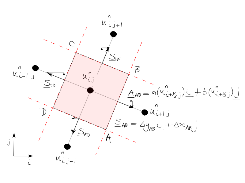
1.1.9.5.4.4. Upwind Scheme: Cell Vertex¶

\[\text{if} (\mathbf{A} \cdot \mathbf{S})_{AB} \gt 0 \quad (\mathbf{F} \cdot \mathbf{S})_{AB} = (\mathbf{F} \cdot \mathbf{S})_{CD}\]

\[\text{if} (\mathbf{A} \cdot \mathbf{S})_{AB} \lt 0 \quad (\mathbf{F} \cdot \mathbf{S})_{AB} = (\mathbf{F} \cdot \mathbf{S})_{EF}\]

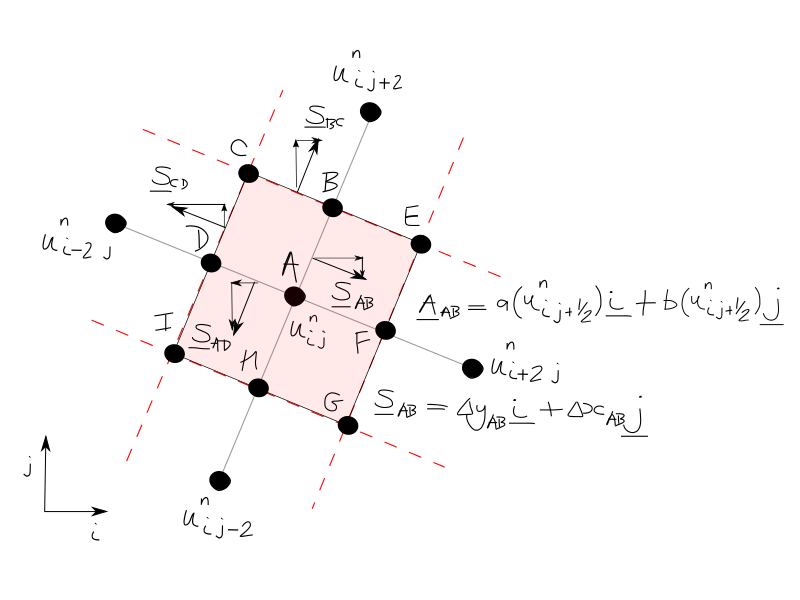
Control volume is ABCDEFGHI

Problem with cell vertex scheme: Contains contributions from \(i+2, j\) and \(i-2, j\) etc i.e. a wide stencil - so not used in practice

1.1.9.5.5. Example of Upwind on a Cartesian Mesh¶

Where: \(a, b \gt 0\) (i.e. the Jacobian is always positive)

Fluxes: \(f = au\) and \(g = bu\)

Vertical sides AB, CD:

Horizontal sides DA, BC:

Resulting scheme (recovered first order upwind):

Or:

Equivalence to first order upwind implies leading truncation error will cause numerical diffusion

We do not require that the mesh is Cartesian

1.1.9.5.6. Summary of FVM¶

• General and flexible:

• arbitary geometry

• any mesh

• Uses integral formulation of the governing equations (does not assume continuous solution), this is closer to the physics

• can have shocks

• interfaces

• any discontinuity

• Conservative discretisation (numerical flux is conserved between control volumes):

• good for strong gradients

• When applied to Cartesian meshes, FV method recovers the FD formulas - can look at convergence properties more easily

• Evaluation of fluxes determines scheme (in FVM we are using FD to evaluate the fluxes on the faces of the FV):

• Central: based on local flux estimation (2nd order) but can’t identify direction of flow

• Upwind: according to direction of propagation, but it’s 1st order

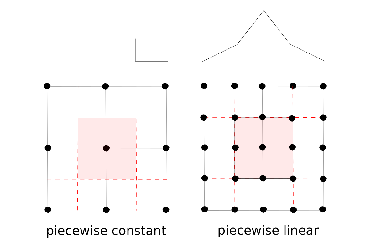
• Interpolation is implied in the discretisation, either piecewise constant or piecewise linear:

• Volumes need not coincide with mesh cells:

  • Mesh cells cannot overlap

  • Volumes are where the conservation laws are applied - these can overlap

  • Decoupling of volumes and cells gives more flexibility than FDM and FEM

1.1.9.5.7. Difficulties with FVM¶

• Accurate definition of derivatives:

• the computational grid is not necessarily orthogonal or equally spaced

• a definition of derivatives using Taylor series is not possible

• Difficult to obtain higher order accuracy:

• representation of function values or fluxes is piecewise constant or piecewise linear, anything more than this is complex

• most FVMs are at most 2nd order (usually sufficient)

• 2 levels of approximation - interpolation and integration determine the order of accuracy

• Data on boundaries:

• cell-centred - data needs to be extrapolated

• cell-vertex - averaging - the flux through a volume surface is smooth

1.1.9.5.8. FVM Approximation of Derivatives¶

1.1.9.5.8.2. General procedure¶

Gauss divergence theorem - think of defining an average of the gradient of a scalar function \(u\) as a function of the values at the boundary. For a vector field:

\[\int_{\Omega} (\mathbf{\nabla} \cdot \mathbf{F}) d \Omega = \oint_S \mathbf{F} \cdot \mathbf{n} d S\]

Or if S is the vector:

\[\int_{\Omega} (\mathbf{\nabla} \cdot \mathbf{F}) d \Omega = \int_{\Omega} (\text{div } \mathbf{F}) d \Omega = \oint_S \mathbf{F} \cdot d \mathbf{S}\]

For a scalar field, replacing \(\mathbf{F}\) with the scalar \(u\)

\[\int_{\Omega} (\mathbf{\nabla} u) d \Omega = \int_{\Omega} (\text{grad } u) d \Omega = \oint_S u \cdot d \mathbf{S}\]

Define the average gradient as:

\[\left({ {\partial \overline{u}} \over {\partial x} } \right)_{\Omega} = {1 \over \Omega} \int_{\Omega} {{\partial u} \over {\partial x}} d \Omega = {1 \over \Omega} \oint_{S} u dy\]

\[\left({ {\partial \overline{u}} \over {\partial y} } \right)_{\Omega} = {1 \over \Omega} \int_{\Omega} {{\partial u} \over {\partial y}} d \Omega = {1 \over \Omega} \oint_{S} u dx\]

In 2D, cell-centered approach:

\[\left({ {\partial \overline{u}} \over {\partial x} } \right)_{X} = {1 \over \Omega} \oint_{S} u dy\]

Integrate over the shaded volume to get the derivative at X

Using the Trapezoidal rule: “Half the sum of the parallel sides times the distance between them”

\[\int_a^b f(y) dy = {{f(a) + f(b)} \over 2} (b - a)\]

Hence:

\[\begin{split}\left({ {\partial \overline{u}} \over {\partial x} } \right)_{X} = {1 \over {2 \Omega}} \left( (u_{i+1,j+1}+u_{i,j+1})(y_{i,j+1}-y_{i+1,j+1}) + \\ (u_{i,j+1}+u_{i,j})(y_{i,j}-y_{i,j+1})+ \\ (u_{i,j}+u_{i+1,j})(y_{i+1,j}-y_{i,j})+ \\ (u_{i+1,j}+u_{i+1,j+1})(y_{i+1,j+1}-y_{i+1,j}) \right)\end{split}\]

Hence:

\[\begin{split}\left({ {\partial \overline{u}} \over {\partial x} } \right)_{X} = {1 \over {2 \Omega}} \left( u_{i+1,j+1}(y_{i,j+1}-y_{i+1,j}) + \\ u_{i,j+1}(y_{i,j}-y_{i+1,j+1})+ \\ u_{i,j}(y_{i+1,j}-y_{i,j+1})+ \\ u_{i+1,j}(y_{i+1,j+1}-y_{i,j}) \right)\end{split}\]

Where the volume \(\Omega\) is given by half the area of a parallelogram:

\[\Omega = {1 \over 2}(y_{i+1,j+1}-y_{i,j})(x_{i+1,j}-x_{i,j+1}) + {1 \over 2}(y_{i,j+1}-y_{i+1,j})(x_{i+1,j+1}-x_{i,j})\]