1.1.9.3. 2D Finite Volume Method: Spatial and Numerical Discretisation
1.1.9.3.1. Spatial Discretisation
1.1.9.3.1.1. Types of Spatial Discretisation
The FVM can handle any type of spatial discretisation
For the same mesh we can have different definitions of the control volumes:
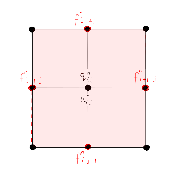
Cell-centred scheme
Control volumes are identical with the grid cells
Flow variables are located at the centres of grid cells - \(q_{i,j}\) and \(u_{i,j}\) can be an average
Fluxes are located at the volume surfaces (red)

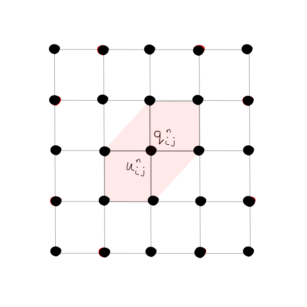
Cell-vertex scheme
Control volume is 4 cells that share the grid point \(i,j\)
Control volumes may overlap
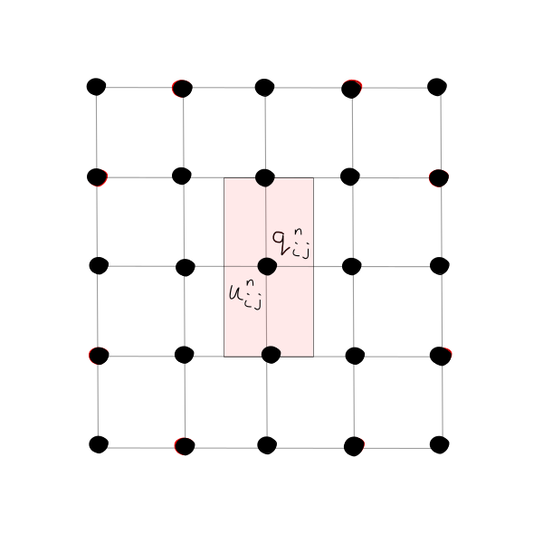
Hexagonal control volume scheme
Trapezoidal control volume scheme
1.1.9.3.1.2. For a Consistent Scheme
The sum of all CVs should cover the entire domain
The sub-domains \(\Omega_J\) are allowed to overlap, as long as each portion of the surface \(S_J\) have to appear as a part of an even number of different surfaces - so that the fluxes cancel out, e.g. 2 surfaces, 4 surfaces etc.
Computing fluxes along a cell surface has to be independent of the cell in which they are considered - ensures that conservation is satisfied
1.1.9.3.2. Numerical Discretisation
Apply integral conservation law to subvolumes (\(\Omega_J\) = sub-volume, \(S_J\) = sub-surface)
Discrete Form, for small volumes (J)
Where:
\(\overline{U_J}\) and \(\overline{Q_J}\) are averaged values over the cell
If integrating between time level \(n\) and \(n+1\), then using 1st order Euler (we could use Runge-Kutta etc)
What are the Cell Averaged Values and the Star Values?
Cell-Averaged Values
Star Values
The reason we omitted the time index in (3) for the balance of fluxes and the sources was to indicate the choice:
If \(n\) was chosen, it would have been an explicit scheme
If \(n+1\) was chosen it would have been an implicit scheme
A scheme is identified by the way the numerical flux \(\mathbf{F^*}\) approximates the time averaged physical flux across each cell face.
Leaving open the choice of time integrator:
RHS defines the “residual” \(R_J\)