1.1.9.2. Conservative Discretisation
1.1.9.2.1. Definition of a Conservation Law
Recall - what is a conservation law?
“Conservation means the variation of a conserved (intensive) flow quantity within a given volume is due to the net effect of some internal sources and the amount of that quantity which is crossing the boundary surface”
Essentially we are looking at the net effect of:
Sources
Fluxes
1.1.9.2.1.1. How to Identify Fluxes
Fluxes appear exclusively under the gradient operator - the flux is the only spatial derivative that appears in the equation
This is a way to recognise if flux is conserved - look at the gradient operator - can you group the spatial derivatives under a gradient operator, so that the fluxes have divergence - i.e. a measure of “outgoingness”?
In conservative form, we usually have mass flux, momentum flux and total energy flux
1.1.9.2.1.2. How to Identify Sources
Sources are usually scalars in one direction and don’t usually have divergence, e.g. gravity, pressure gradient
1.1.9.2.2. Differential Discretisation
The differential form requires the fluxes to be differentiable - this is not always satisfied, this may introduce impossible solutions.
Discontinuities introduce infinite gradient, e.g.
shocks in the flow
a free surface
a slip line behind a trailing edge
1.1.9.2.3. Conservative Discretisation
1.1.9.2.3.1. General Form of a Conservation Law
where:
\(\Omega =\) volume
\(S =\) surface
\(U =\) quantity
\(F =\) flux vector
\(Q =\) source
i.e. the quantity \(U\) only depends on the surface values of the fluxes
1.1.9.2.3.2. Conservative Discretisation
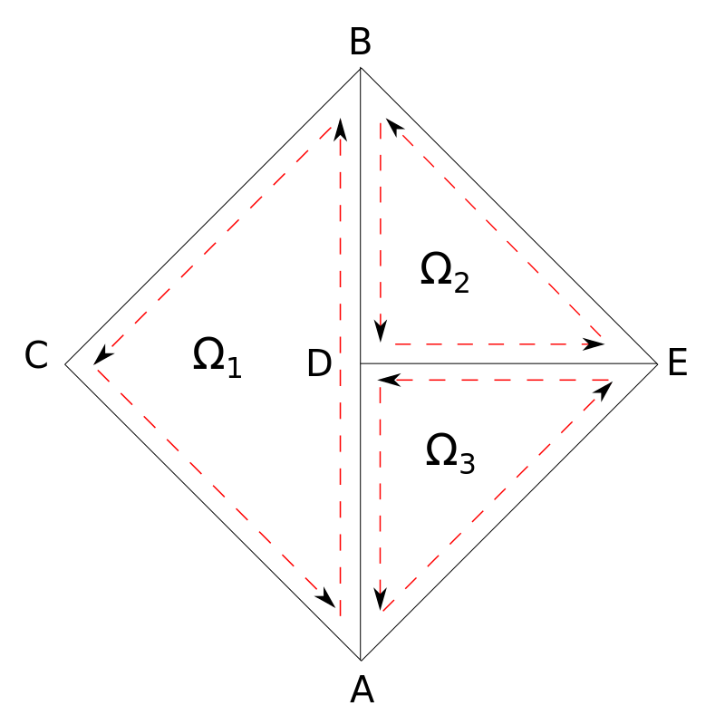
\(\Omega\) divided into \(\Omega_1\), \(\Omega_2\) and \(\Omega_3\):
For each subvolume:
Notice that the contribution of the internal fluxes, cancel each other out when summated in each direction. Hence the numerical scheme is conservative in the way it treats the flux terms.
1.1.9.2.3.3. Example of Conservative Discretisation
Consider a 1D conservation law in conservative form:

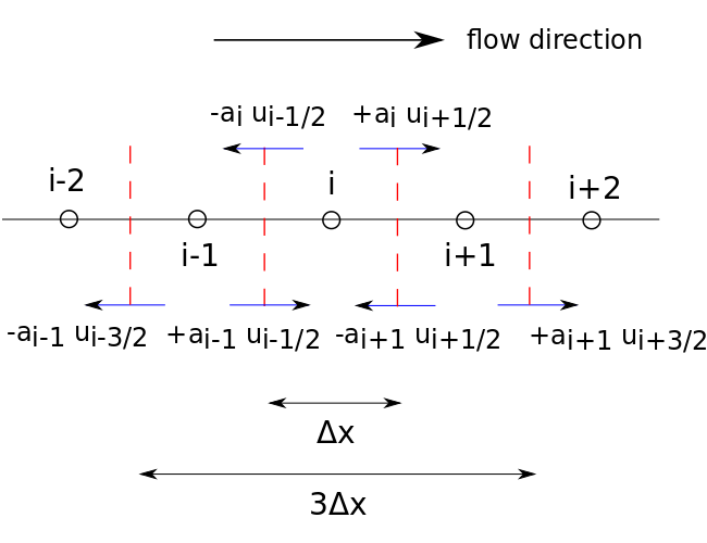
Associate a finite “cell” to each mesh point, e.g. cell (i) has two “cell faces” at the mid-points \(i-{1/2}\) and \(i+{1/2}\)
Using a CD scheme at point i:
Using a CD scheme at point i+1:
Using a CD scheme at point i-1:
Add (1), (2) and (3) and divide by 3 for a consistent discretisation of the conservation law for cell \(i-3/2\) to \(i+3/2\):
A scheme applied directly to cell \(i-3/2\) to \(i+3/2\):
The flux of (4) and (5) are identical, but the difference is that the flow quantity and source terms are averaged over three mesh points in (4)
1.1.9.2.3.4. Example of Non-Conservative Discretisation
Consider a 1D conservation law in conservative form:
where:
\(a(u)\) is the Jacobian and \(a = \partial f / \partial u\)
(e.g. Burgers \(a=u\), \(f=u^2 / 2\))
Using a CD scheme at point i:
Using a CD scheme at point i+1:
Using a CD scheme at point i-1:
Add (6), (7) and (8) and divide by 3 for an consistent discretisation of the conservation law for cell \(i-3/2\) to \(i+3/2\):
Reconstruct what we would want on the LHS, and put the remainder on the RHS:
The extra terms on the RHS of (10) result from the fact that the flux contributions at the internal points of the cell \(i-3/2\) to \(i+3/2\) do not cancel
They appear as additional source terms
The discretisation of the non-conservative form of the equation leads to internal sources
The Conservative and Non-Conservative forms of the equations are mathematically equivalent for arbitrary non-linear fluxes
But they are not numerically equivalent
The Taylor expansion of the source terms shows that they are like a 2nd order discretisation proportional to \(\Delta x^2(a_x u_x)_x\) (same order as the truncation error)
Numerical experiments show that the non-conservative form is less accurate than the conservative form, especially for discontinuous flows (e.g. shocks) where the gradient is very large, the numerical source terms can become important.