1.2.1.5. 2D First-order Linear Convection
1.2.1.5.1. Understand the Problem
What is the final velocity profile for 2D linear convection when the initial conditions are a square wave and the boundary conditions are unity?
2D linear convection is described as follows:
1.2.1.5.2. Formulate the Problem
1.2.1.5.2.1. Input Data
nt = 51 (number of temporal points)
tmax = 0.5
nx = 21 (number of x spatial points)
nj = 21 (number of y spatial points)
xmax = 2
ymax = 2
c = 1
Initial Conditions: \(t=0\)
x |
i |
y |
j |
u(x,y,t), v(x,y,t) |
|---|---|---|---|---|
\(0\) |
\(0\) |
\(0\) |
\(0\) |
\(1\) |
\(0 < x \le 0.5\) |
\(0 < i \le 5\) |
\(0 < y \le 0.5\) |
\(0 < j \le 5\) |
\(1\) |
\(0.5 < x \le 1\) |
\(5 < i \le 10\) |
\(0.5 < y \le 1\) |
\(5 < j \le 10\) |
\(2\) |
\(1 < x < 2\) |
\(10 < i < 20\) |
\(1 < y < 2\) |
\(10 < j < 20\) |
\(1\) |
\(2\) |
\(20\) |
\(2\) |
\(20\) |
\(1\) |
Boundary Conditions: \(x=0\) and \(x=2\), \(y=0\) and \(y=2\)
t |
n |
u(x,y,t), v(x,y,t) |
|---|---|---|
\(0 \le t \le 0.5\) |
\(0 \le n \le 50\) |
\(1\) |
1.2.1.5.2.2. Output Data
x |
y |
t |
u(x,y,t), v(x,y,t) |
|---|---|---|---|
\(0 \le x \le 2\) |
\(0 \le y \le 2\) |
\(0 \le t \le 0.5\) |
\(?\) |
1.2.1.5.3. Design Algorithm to Solve Problem
1.2.1.5.3.1. Space-time discretisation
i \(\rightarrow\) index of grid in x
j \(\rightarrow\) index of grid in y
n \(\rightarrow\) index of grid in t
1.2.1.5.3.2. Numerical scheme
FD in time
BD in space
1.2.1.5.3.3. Discrete equation
1.2.1.5.3.4. Transpose
1.2.1.5.3.5. Pseudo-code
#Constants
nt = 51
tmax = 0.5
dt =  tmax/(nt-1)
nx =  21
xmax = 2
ny = 21
ymax = 2
dx = xmax/(nx-1)
dy = ymax/(ny-1)

#Boundary Conditions
for n between 0 and 50
   for i between 0 and 20
      u(i,0,n)=v(i,0,n)=1
      u(i,20,n)=v(i,20,n)=1
   for j between 0 and 20
      u(0,j,n)=v(0,j,n)=1
      u(20,j,n)=v(20,j,n)=1

#Initial Conditions
for i between 1 and 19
   for j between 1 and 19
      if(5 < i < 10 OR 5 < j < 10)
         u(i,j,0) = v(i,j,0)= 2
      else
         u(i,j,0) = v(i,j,0)= 1

#Iteration
for n between 0 and 49
   for i between 1 and 19
      for j between 1 and 19
          u(i,j,n+1) = u(i,j,n)-c*dt*[(1/dx)*(u(i,j,n)-u(i-1,j,n))+
                                      (1/dy)*(u(i,j,n)-u(i,j-1,n))]
          v(i,j,n+1) = v(i,j,n)-c*dt*[(1/dx)*(v(i,j,n)-v(i-1,j,n))+
                                      (1/dy)*(v(i,j,n)-v(i,j-1,n))]
1.2.1.5.4. Implement Algorithm in Python
def convection(nt, nx, ny, tmax, xmax, ymax, c):
   """
   Returns the velocity field and distance for 2D linear convection
   """
   # Increments
   dt = tmax/(nt-1)
   dx = xmax/(nx-1)
   dy = ymax/(ny-1)

   # Initialise data structures
   import numpy as np
   u = np.ones(((nx,ny,nt)))
   v = np.ones(((nx,ny,nt)))
   x = np.zeros(nx)
   y = np.zeros(ny)

   # Boundary conditions
   u[0,:,:] = u[nx-1,:,:] = u[:,0,:] = u[:,ny-1,:] = 1
   v[0,:,:] = v[nx-1,:,:] = v[:,0,:] = v[:,ny-1,:] = 1

   # Initial conditions
   u[int((nx-1)/4):int((nx-1)/2),int((ny-1)/4):int((ny-1)/2),0]=2
   v[int((nx-1)/4):int((nx-1)/2),int((ny-1)/4):int((ny-1)/2),0]=2

   # Loop
   for n in range(0,nt-1):
      for i in range(1,nx-1):
         for j in range(1,ny-1):
            u[i,j,n+1] = (u[i,j,n]-c*dt*((1/dx)*(u[i,j,n]-u[i-1,j,n])+
                                         (1/dy)*(u[i,j,n]-u[i,j-1,n])))
            v[i,j,n+1] = (v[i,j,n]-c*dt*((1/dx)*(v[i,j,n]-v[i-1,j,n])+
                                         (1/dy)*(v[i,j,n]-v[i,j-1,n])))

   # X Loop
   for i in range(0,nx):
      x[i] = i*dx

   # Y Loop
   for j in range(0,ny):
      y[j] = j*dy

   return u, v, x, y

def plot_3D(u,x,y,time,title,label):
   """
   Plots the 2D velocity field
   """

   import matplotlib.pyplot as plt
   import numpy as np
   from mpl_toolkits.mplot3d import Axes3D
   fig=plt.figure(figsize=(11,7),dpi=100)
   ax=fig.gca(projection='3d')
   ax.set_xlabel('x (m)')
   ax.set_ylabel('y (m)')
   ax.set_zlabel(label)
   X,Y=np.meshgrid(x,y)
   surf=ax.plot_surface(X,Y,u[:,:,time],rstride=2,cstride=2)
   plt.title(title)
   plt.show()
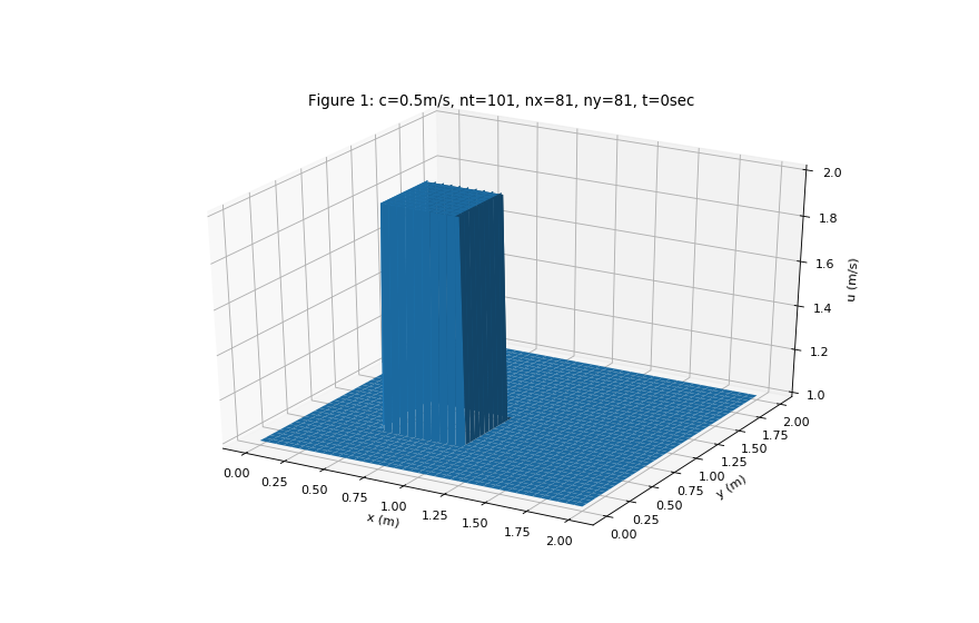
u,v,x,y = convection(101, 81, 81, 0.5, 2.0, 2.0, 0.5)
plot_3D(u,x,y,0,'Figure 1: c=0.5m/s, nt=101, nx=81, ny=81, t=0sec','u (m/s)')
plot_3D(u,x,y,100,'Figure 2: c=0.5m/s, nt=101, nx=81, ny=81, t=0.5sec','u (m/s)')
plot_3D(v,x,y,0,'Figure 3: c=0.5m/s, nt=101, nx=81, ny=81, t=0sec','v (m/s)')
plot_3D(v,x,y,100,'Figure 4: c=0.5m/s, nt=101, nx=81, ny=81, t=0.5sec','v (m/s)')


1.2.1.5.5. Conclusions
1.2.1.5.5.1. Why isn’t the square wave maintained?
As with 1D, the first order backward differencing scheme in space creates false diffusion.
1.2.1.5.5.2. Why does the wave shift?
The square wave is being convected by the constant linear wave speed c in 2 dimensions
For \(c > 0\) profiles shift by \(c \Delta t\) - compare Figure 1, 2, 3 and 4