3.1.6.1.1. Non-linear Breaking Waves in Shallow Water¶

• This paper has an important application to non-linear breaking waves in shallow water. The approach taken in this category follows the fully non-linear equations for a deterministic time-resolving model for one realisation of wave frequency, similar to the approach of Ravel et al (2009). However, unlike Ravel, the numerical method used reformulates the convective mass fluxes in order to allow highly non-linear behaviour at the interface. This allows breaking waves to be considered, which was not considered by Ravel et al (2009).

• It is known in the wave modelling community that as the water depth reduces, wave breaking becomes an important phenomenon. However, there is also the simultaneous effect of bottom friction, and it is difficult to separate the effect of bottom friction from the effect of wave breaking in shallow water. Although this study focusses mainly on wave breaking, it follows the approach outlined by Cavaleri et al (2007) in which wave breaking and bottom friction could be studied together if needed.

• The time resolving approach may be better suited to non-linear breaking in shallow water compared with stochastic methods because of the highly non-linear and dissipative effects that are present. However, there is an inherent computational penalty of the time-resolving approach as multiple realisations may be needed.

3.1.6.1.2. Numerics¶

• This study is also in the class of numerics, attempting to minimise the numerical errors created due to the description of the flow field.

• The approach has the potential to introduce less numerical error compared to the arithmetic mean approach for the density term in the convective mass fluxes of say Zwart, Burns and Galpin (2007).

• The approach is 2D, such that the wet-dry areas are really wet-dry lengths, but most numerical simulations of this type are 2D.

3.1.6.3.1. Problems¶

1. Instantaneous density jump across a free surface - use conservative integral form of Navier-Stokes because density in convection term stays inside integrand

2. Computing accurate velocity field, hence shear stress for wind blowing over waves - use finite volume method to ensure conservation of mass and momentum

3.1.6.3.2. Purposes¶

Purpose 1: Explore conservative integral form for free surface flows

• The conservative integral form of the Navier-Stokes equations has been used in the cut-cell method - to cut solid boundaries from the Cartesian grid to include only fluid in the calculation

• High resolution Godunov scheme was used for free surface flows to calculate density and velocity

• Cut cell method has been used to cut air out of the solution

Purpose 2: Accurately calculate mass fluxes using standard staggered grid

• Mass fluxes passing through the u and v control volumes are the most important

• For co-located grids, mass fluxes on the f control volumes have been for the mass fluxes on the u and v control volumes before

• For staggered grids, more difficult to get u and v fluxes from f flux - can use an f-grid that is twice as fine as the u and v grid - but this is not standard

Other features

• Second order scheme for time derivatives

• High-resolution scheme for interpolation of velocity onto the surface of the control volume

• Second order scheme for viscous terms

• SIMPLEC-PISO scheme for pressure-velocity coupling

• Explicit high resolution compressive interface capturing scheme for arbitrary meshes (CICSAM) for predicting the volume fraction of the fluid

3.1.6.4.1. Governing Equations¶

• Volume Conservation:

• Mass Conservation:

• Momentum Conservation for \(u\):

• Momentum Conservation for \(v\):

• Volume Fraction Conservation:

where:

\(\mathbf n = n_x \mathbf i + n_y \mathbf j = \begin{bmatrix} 1 & 0 \end{bmatrix} \text{for east surface}, \begin{bmatrix} 0 & 1 \end{bmatrix} \text{for north surface}, \begin{bmatrix} -1 & 0 \end{bmatrix} \text{for west surface}, \begin{bmatrix} 0 & -1 \end{bmatrix} \text{for south surface}\)

\(\mathbf v = u \mathbf i + v \mathbf j\) = \(\begin{bmatrix} u \\ v \end{bmatrix}\)

\(n_x = 1 \text{ for east surface}, -1 \text{ for west surface}\), \(n_y = 1 \text{ for north surface}, -1 \text{ for south surface}\)

\({\partial \over \partial n} = {\partial \over \partial x} \text{ for east surface}, -{\partial \over \partial x} \text{ for west surface}\), \({\partial \over \partial y} \text{ for north surface}, -{\partial \over \partial y} \text{ for south surface}\)

Unknowns:

• Velocities \(u\) and \(v\)

• Pressure \(p\)

• Volume fraction \(f\)

3.1.6.4.2. Discretisation of Governing Equations¶

Aim: Obtain an algebraic formulation for velocities at centre of control volume \(u_P\) and \(v_P\)

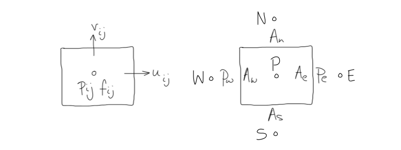
LHS: Staggered Location for \(u, v, p\) and \(f\) RHS: \(u\) control volume

Discrete Mass Conservation Equation

Mass Conservation Equation (2) - all values are at time n+1

Discrete Momentum Conservation Equation for \(u\)

Momentum Conservation Equation (3) - all values are at time n+1

3.1.6.4.3. Apply Numerical Schemes¶

3.1.6.4.3.2. Velocity Terms at Faces: Blended Scheme¶

(12)¶\[u_e = u_P + \beta {{u_P-u_W} \over 2}\]

where for flow in +ve x-direction: \(\beta = 0 \text{ (1st order upwind)}\) \(\beta = {{u_E-u_P} \over {u_P-u_W}} \text{ (central)}\) and \(\beta = 1 \text{ (2nd order upwind)}\)

For flow in other directions:

Face velocity	+ve upwind	-ve upwind	Central	+ve 2nd order upwind	-ve 2nd order upwind
\(u_e\)	\(u_P\)	\(u_E\)	\({u_P+u_E} \over 2\)	\({3u_P-u_W} \over 2\)	\({3u_E-u_{EE}} \over 2\)
\(u_w\)	\(u_W\)	\(u_P\)	\({u_W+u_P} \over 2\)	\({3u_W-u_{WW}} \over 2\)	\({3u_P-u_E} \over 2\)
\(u_n\)	\(u_P\)	\(u_N\)	\({u_P+u_N} \over 2\)	\({3u_P-u_S} \over 2\)	\({3u_N-u_{NN}} \over 2\)
\(u_s\)	\(u_S\)	\(u_P\)	\({u_S+u_P} \over 2\)	\({3u_S-u_{SS}} \over 2\)	\({3u_P-u_N} \over 2\)

Simplification to 1st order upwind scheme (to illustrate numerical scheme)

\(F_e > 0 \Rightarrow u_e = u_P\)

\(F_e < 0 \Rightarrow u_e = u_E\)

(13)¶\[F_e u_e = u_P \begin{bmatrix}F_e, & 0 \end{bmatrix} - u_E\begin{bmatrix}-F_e, & 0 \end{bmatrix}\]

where \(\begin{bmatrix} F_e, & 0 \end{bmatrix}\) means the maximum of \(F_e\) and 0

Similarly:

(14)¶\[F_w u_w = u_W \begin{bmatrix}F_w, & 0 \end{bmatrix} - u_P\begin{bmatrix}-F_w, & 0 \end{bmatrix}\]

(15)¶\[F_n u_n = u_P \begin{bmatrix}F_n, & 0 \end{bmatrix} - u_N\begin{bmatrix}-F_n, & 0 \end{bmatrix}\]

(16)¶\[F_s u_s = u_S \begin{bmatrix}F_s, & 0 \end{bmatrix} - u_P\begin{bmatrix}-F_s, & 0 \end{bmatrix}\]

3.1.6.5.1. u-control volume¶

Determine the Flux Terms by considering the Convective Term for the North Face:

Similarly:

What value do the terms \(L_a\) and \(L_w\) have?

Outward Normal Vector

Negative sign indicates that the change in volume fraction in the positive x and y directions is negative

• Case 1: \(-{{\partial f} \over {\partial y}}>0\) and \(\left\vert{{\partial f} \over {\partial y}}\right\vert>\left\vert{{\partial f} \over {\partial x}}\right\vert\)

• Case 2: \(-{{\partial f} \over {\partial y}}<0\) and \(\left\vert{{\partial f} \over {\partial y}}\right\vert>\left\vert{{\partial f} \over {\partial x}}\right\vert\)

• Case 3: \(-{{\partial f} \over {\partial x}}>0\) and \(\left\vert{{\partial f} \over {\partial x}}\right\vert>\left\vert{{\partial f} \over {\partial y}}\right\vert\)

• Case 4: \(-{{\partial f} \over {\partial x}}<0\) and \(\left\vert{{\partial f} \over {\partial x}}\right\vert>\left\vert{{\partial f} \over {\partial y}}\right\vert\)

Now we only need to calculate the wet dry areas case 1, and then rotate it’s orientation for the other cases.

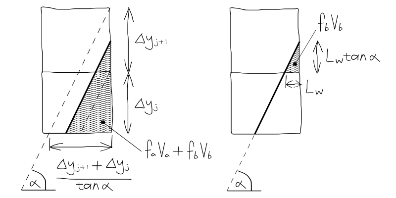
3.1.6.5.1.1. \(L_w\) and \(L_a\) where \(tan(\alpha) < \Delta y / \Delta x\) on north face¶

Consider Case 1

Compute for each u and v control volume:

• Wet area

• Dry area

• Viscosity on each face

• Total mass

Assumptions:

• Angle between unit vector \(\mathbf n\) and positive y axis is in the range -45 degrees to +45 degrees

• Bottom to top, \(f\) and \(\mu\) are discontinuous

• Left to right, the \(f\) is a continous function and conventional interpolation or averaging can be applied

• Air-water interface is a straight line in control volume

(19)¶\[tan(\alpha) = \left \vert {{(f_{i+1,j+1}+f_{i+1,j}-f_{i,j+1}-f_{i,j})\Delta y} \over {(f_{i,j+1}+f_{i+1,j+1}-f_{i,j}-f_{i+1,j})\Delta x}} \right \vert\]

A table might also clarify:

Case	\(f_{i,j}\)	\(f_{i+1,j}\)	\(f_{i,j+1}\)	\(f_{i+1,j+1}\)	\(tan(\alpha)\)	\(\alpha\)
1	1	0.5	0.5	0	\(\left \vert 1 \right \vert\)	45
2	0	0.5	0.5	1	\(\left \vert 1 \right \vert\)	45
1 flipped horizontally	0.5	1	0	0.5	\(\left \vert -1 \right \vert\)	45
2 flipped horizontally	0.5	0	1	0.5	\(\left \vert -1 \right \vert\)	45

The volume fraction is continuous from left to right, so the standard average process is applied:

(20)¶\[f_a = {{f_{i+1,j}+f_{i,j}} \over 2}\]

(21)¶\[f_b = {{f_{i+1,j+1}+f_{i,j+1}} \over 2}\]

\(f\) is defined as:

\[f = {{\text{area of water}} \over {\text{area of cell}}}\]

\(1-f\) is defined as:

\[1-f = {{\text{area of air}} \over {\text{area of cell}}}\]

For similar triangles:

\[\left ( {{\text{length of water}} \over {\text{length of air}}} \right )^2 = {{\text{area of water}} \over {\text{area of air}}}\]

Hence:

\[\left ( {L_w} \over {L_a} \right )^2 = {{f_b \Delta x \Delta y_{j+1}} \over {(1-f_a) \Delta x \Delta y_{j}}}\]

Solution for \(L_w\)

(22)¶\[L_w = {({f_b \Delta y_{j+1})^{0.5}} \over {{(f_b \Delta y_{j+1})^{0.5}} + ((1-f_a) \Delta y_{j})^{0.5} }}\]

Solution for \(L_a\)

(23)¶\[L_a = \Delta x - L_w\]

From Equation (22) and (23)

• If \(f_b = 0\) and \(f_a = 1\) then \(L_w = 0\) and \(L_a = \Delta x\)

• If \(f_b = 1\) and \(f_a = 0\) then \(L_w = \Delta x\) and \(L_a = 0\)

Advantages of Equation (22):

• We don’t need to know that the interface is between P and N for Equation (22)

• We don’t need the angle \(\alpha\)

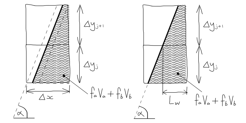
3.1.6.5.1.2. \(L_w\) and \(L_a\) where \(tan(\alpha) > \Delta y / \Delta x\) on north face¶

Case A solution for \(L_w\) ( \(L_a\) from equation (23) )

\[\begin{split}f_a V_a + f_b V_b \leqslant {{(\Delta y_j)^2} \over {2 tan \alpha}} \\\end{split}\]

(24)¶\[L_w = 0\]

\[f_b = 0\]

Case B solution for \(L_w\) ( \(L_a\) from equation (23) )

\[{{(\Delta y_j)^2} \over {2 tan \alpha}} \le f_a V_a + f_b V_b \le {{(\Delta y_j + \Delta y_{j+1})^2} \over {2 tan \alpha}}\]

Area of a triangle:

(25)¶\[L_w = \left ({2 f_b V_b} \over {tan \alpha} \right )^{0.5}\]

Case C solution for \(L_w\) ( \(L_a\) from equation (23) )

\[{{(\Delta y_j + \Delta y_{j+1})^2} \over {2 tan \alpha}} \le f_a V_a + f_b V_b \le (\Delta y_{j+1} + \Delta y_{j}) \Delta x- {{(\Delta y_j + \Delta y_{j+1})^2} \over {2 tan \alpha}}\]

From the area of a trapezoid:

(26)¶\[L_w = {{f_a V_a + f_b V_b} \over {\Delta y_j + \Delta y_{j+1}}}\]

Case D solution for \(L_w\) (this is just Case B but rotated 180 degrees and i.t.o. air \(L_a\) from equation (23) )

From Case B (i.t.o. air):

\[{{(\Delta y_{j+1})^2} \over {2 tan \alpha}} \le (1-f_a) V_a + (1-f_b) V_b \le {{(\Delta y_j + \Delta y_{j+1})^2} \over {2 tan \alpha}}\]

From the area of a triangle:

(27)¶\[L_w = \Delta x - \left ({2 (1-f_a) V_a} \over {tan \alpha} \right )^{0.5}\]

Case E solution for \(L_w\) (this is just Case A but rotated 180 degrees and i.t.o. air \(L_a\) from equation (23) )

From Case A (i.t.o. air):

\[(1-f_a) V_a + (1-f_b) V_b \le {({\Delta y_{j+1})^2} \over {2 tan \alpha}}\]

From the area of a triangle:

(28)¶\[L_w = \Delta x\]

\[f_a = 1\]

3.1.6.5.1.4. \(\mu\) on north face (\(\mu_n\))¶

What do we need to compute?

The diffusive flux on the north face:

\[D_n = \mu_n {{A_n} \over {\Delta y_n}}\]

What is \(\mu_n\)?

• We are concerned with the viscosity at the interface between points P and N.

• As Patankar (1980) suggests, we must determine the distance to the interface from the points P and N.

• The governing assumption here is that very steep angles > 45 degrees or < -45 degrees are not present

• Note that this assumption only applies to the viscosity and not to the convective flux, which does allow sharp angles

• The second governing assumption is that the viscosity at the interface is represented by the harmonic mean, so significant variation in the viscosity (e.g. due to turbulence) between the grid points at the interface is negligible

The use of the harmonic mean follows the suggestion of Patankar (1980) who used it for non-uniform conductivity in the diffusive term. Patankar (1980) dismisses the use of the arithmetic mean as too simplistic, but he did not consider the geometric mean or the infinite norm mean see Schmeling et al (2008). We also don’t know whether turbulent viscosity can be best represented by these averaging methods.

There are four cases:

• \(f_a < 0.5\) and \(f_b = 0\) so \(d_w = 0\)

• \(f_a > 0.5\) and \(f_b = 0\) so \(d_w = (f_a - 0.5)\Delta y_j\)

• \(f_a > 0.5\) and \(f_b < 0.5\) so \(d_w = {(f_a - 0.5)\Delta y_j} +f_b \Delta y_{j+1}\)

• \(f_a > 0.5\) and \(f_b > 0.5\) so \(d_w = {(f_a - 0.5)\Delta y_j} +0.5 \Delta y_{j+1}\)

This can be summarized like this, where \(d_w\) is the distance from P to the interface:

(30)¶\[d_w = max(f_a-0.5,0)\Delta y_j + min(f_b,0.5)\Delta y_{j+1}\]

The distance from N to the interface is \(d_a\) and this is simply the distance between P and N minus \(d_w\):

(31)¶\[d_a = {{\Delta y_j + \Delta y_{j+1}} \over 2} - d_w\]

Harmonic Mean Viscosity

This is how Patankar (1980) defines the harmonic mean viscosity (for the north face):

(32)¶\[\mu_n = \left ( {f_w \over \mu_w} + {f_a \over \mu_a} \right )^{-1}\]

Where:

(33)¶\[f_w = {d_w \over {d_a + d_w}}\]

And:

(34)¶\[f_a = {d_a \over {d_a + d_w}}\]

Substituting Equation (33) and (34) into (32) and re-arranging gives:

(35)¶\[\mu_n ={ {\mu_w \mu_a (d_w + d_a)} \over {\mu_a d_w + \mu_w d_a}}\]

3.1.6.5.2. v-control volume¶

The angle \(\alpha\) is from Brackbill et al (1994) - I’m not sure why the angle the interface makes with the x-axis would be different for the v control volume? Or why we would need another equation for the same value? Is this because the v-volume fraction is stored at the faces and not the cell centres?

Why isn’t this the same as Equation (19)?

3.1.6.5.2.1. \(L_w\) and \(L_a\) where \(tan(\alpha) < \Delta y / \Delta x\) on north face¶

Case A - Solution for \(L_w\)

\[f_{i,j+1} \le {{\Delta x tan \alpha} \over {2 \Delta y}}\]

\[L_w = 0\]

Case B - Solution for \(L_w\)

\[{{\Delta x tan \alpha} \over {2 \Delta y}} \le f_{i,j+1} \le {1 \over 2} +{{\Delta x tan \alpha} \over {2 \Delta y}}\]

From the area of a trapezoid:

\[L_w = \left ( {{f_{i,j+1}\Delta y } \over {\Delta x tan \alpha} } - {1 \over 2} \right )\]

Case C - Solution for \(L_w\)

\[f_{i,j+1} \ge {1 \over 2} +{{\Delta x tan \alpha} \over {2 \Delta y}}\]

\[L_w = \Delta x\]

3.1.6.5.2.2. \(L_w\) and \(L_a\) where \(tan(\alpha) > \Delta y / \Delta x\) on north face¶

Case A - Solution for \(L_w\)

\[f_{i,j+1} \le {{\Delta y} \over {8 \Delta x tan \alpha}}\]

\[L_w = 0\]

Case B - Solution for \(L_w\)

\[{{\Delta y} \over {8 \Delta x tan \alpha}} \le f_{i,j+1} \le {{\Delta y} \over {2 \Delta x tan \alpha}}\]

From the area of a triangle:

\[L_w ={{(2 \Delta x \Delta y f_{i,j+1} tan \alpha)^{0.5} - {\Delta y \over 2}} \over {tan \alpha}}\]

Case C - Solution for \(L_w\)

\[{{\Delta y} \over {2 \Delta x tan \alpha}} \le f_{i,j+1} \le 1-{{\Delta y} \over {2 \Delta x tan \alpha}}\]

\[L_w = f_{i,j+1} \Delta x\]

Case D - Solution for \(L_w\)

\[1-{{\Delta y} \over {2 \Delta x tan \alpha}} \le f_{i,j+1} \le 1-{{\Delta y} \over {8 \Delta x tan \alpha}}\]

\[L_w = \Delta x + {\Delta y \over {2 tan \alpha}} - {{(2 \Delta x \Delta y (1-f_{i,j+1}) tan \alpha)^{0.5}} \over {tan \alpha}}\]

Case E - Solution for \(L_w\)

\[f_{i,j+1} \ge 1-{{\Delta y} \over {8 \Delta x tan \alpha}}\]

\[L_w = \Delta x\]

Resulting flux

Depending on the value of \(f_{i,j+1}\) and \(\alpha\), the fluid flux produced may vary from:

• \(\rho_a v_n \Delta x\) when \(L_w = 0\) and \(L_a = \Delta x\)

• \(\rho_w v_n \Delta x\) when \(L_w = \Delta x\) and \(L_a = 0\)

3.1.6.5.2.3. \(L_w\) and \(L_a\) on south, east and west faces¶

• Solution for \(L_w\) on south face by replacing \(j\) by \(j-1\) in equations for north face

• Solution for \(L_w\) on east face

\[f_a = {f_{i,j}+f_{i+1,j}}\over 2\]

\[f_b = {f_{i,j+1}+f_{i+1,j+1}}\over 2\]

\[L_w = max(f_a-0.5,0)\Delta y_j+min(f_b,0.5)\Delta y_{j+1}\]

not sure about the following:

\[L_e ={{{ {{\Delta y_{j+1}}}\over 2} + {{\Delta y_{j}}\over 2}} - L_w}\]

• Solution for \(L_w\) on west face by replacing \(i-1\) with \(i\) in equations for east face

3.1.6.5.2.4. \(\mu\) on north face (\(\mu_n\))¶

(37)¶\[d_w = f_{i,j+1} {\Delta y_{j+1}}\]

(38)¶\[d_a = {\Delta y_{j+1}} - d_w\]

I’m not sure about the positioning of the indices, in the above equations

BIG QUESTION: Why is the wet length based on the u-volume fraction cell-centred and the wet length based on the v-volume fraction face-centred?

The harmonic mean is used for the viscosity \(\mu_n\) from Equation (35)

3.1.6.6.1. SIMPLE and SIMPLEC Algorithms¶

• The u momentum equation (17) and v momentum equation (18) are solved iteratively until the normalised residuals are small (perhaps using the tri-diagonal matrix algorithm). At this point we have satisfied momentum conservation.

• However, there is no guarantee that this solution satisfies the volume conservation equation, from equation (1):

• A pressure-correction algorithm is needed in the loop in order to satisfy volume conservation by correcting the following according to the volume conservation equation:

  • velocity

  • pressure

3.1.6.6.2. CICSAM Algorithm¶

• At this point we have satisfied the equations for volume, mass, u momentum and v momentum conservation.

• The final equation to satisfy is the equation for volume fraction conservation (5), which is solved explicitly:

• The values on the surfaces are computed by a high resolution scheme CICSAM. The reason for using CICSAM is that this method is able to produce a sharp water surface

• Normal to the interface, the volume fraction is between 0 and 1 on only one node.

• The problem with Equation (39) is that when the points \(u, w, n, s\) and \(P\) are all in water, the RHS of Equation (39) is:

• Clearly \(f_P\) won’t be exactly 1, so the equation for volume fraction conservation won’t reduce to the equation of volume conservation (which it should in this case). So in solving Equation (39) a correction is applied to the velocity:

• The correction is applied like this to Equation (39)

3.1.6.6.3. CICSAM, SIMPLE-PISO Procedure¶

In order to accelerate convergence, we add a second velocity and pressure produced by the PISO algorithm at the last iteration in each time step

The implicit SIMPLEC-PISO algorithm is combined with the explicit CICSAM algorithm like this:

1. The solution of volume fraction is calculated from the solutions of \(u^n\), \(v^n\) and \(f^n\) by CICSAM.

2. The solutions of \(u\), \(v\) and \(p\) are obtained from the SIMPLEC-PISO algorithm after \(f\) has already been obtained.

3.1.6.7.1. Velocity¶

• Potential flow compares well with the wet-dry areas method in the water, however the difference occurs in the air and near the interface:

  • The velocity field is discontinuous in the potential flow solution, because the viscosity is zero

  • The wet-dry areas method produces a rapid but continuous change in the velocity field

• However remarkably over most of the velocity profile the difference is less than 1%

• The v-velocity variation is continuous in both cases and little difference is seen

3.1.6.7.2. Streamlines¶

• At the peak and trough, streamlines for potential flow are centred at the interface, whereas streamlines for the wet-dry areas method are centred in the air

Generally speaking this exercise of comparing the potential flow solution with the wet-dry areas method was for validation purposes and it showed that sensible results are being produced

I wonder whether a comparison between the standard arithmetic approach to the mass fluxes and the wet-dry areas method would also be useful to compare the shear stress computed at the interface.

3.1.6.10.1. Grid Independence¶

• This was performed for the water column collapse application for T=3.99.

• Uniform, structured grids were used in this case.

• I wonder whether non-uniform structured grids or non-uniform unstructured grids might be more numerically efficient, although they may not be less diffuse.

3.1.6.10.2. The Robustness¶

• The first 20 timesteps of the water column collapse application was also used test robustness.

• The SIMPLEC algorithm used is unconditionally stable, however the convergence at each timestep depends on the timestep - i.e. divergence may occur if the timestep is too large.

• The robustness was tested by using a fixed timestep and testing to see if the volume residual became less than \(5x10^{-4}\)

• The minimum number of iterations per timestep was set to 15, which was achieved quickly after the first five timesteps.

3.1.6.10.3. Efficiency¶

• The efficiency of the wet-dry areas method is less than the average density method due to the use of different cases in the u and v control volumes

• For the water column collapse it is 20% greater (as this uses all 4 cases)

• For the non-linear non-breaking wave and the non-linear breaking wave it is around 10% longer (as these are mainly case 1)