1.1.5.5. Spectral Analysis of Errors¶

von Neumann Stability Analysis
Amplitude and Phase Error
Error Analysis for Hyperbolic Problems
Analysis of 1st Order Upwind
Analysis of Lax-Friedrichs
Analysis of Lax-Wendroff
Summary
Analysis of Leapfrog
What is the Origin of the Oscillations?
Analysis of Beam-Warming
Final Notes
Implications of Diffusion Error for Grid Density
Question

1.1.5.5.1. von Neumann Stability Analysis ¶

von Neumann stability analysis introduced a Fourier decomposition of the solution, defining an amplification factor, G, \(\Rightarrow\) stability condition G < 1
What else can we know about the errors?

Amplitude error \(\Rightarrow\) numerical diffusion

Phase error \(\Rightarrow\) numerical dispersion

We introduced a Fourier decomposition of the solution (where \(I = \sqrt{-1}\)):

\[u_i^n = \sum_{j=-N}^N V_j^n e^{Ik_j x_i} \qquad x_i = i \Delta x\]

A single harmonic is:

\[(u_i^n)_k = V^n e^{I k i \Delta x}\]

We define an amplification factor:

\[G = {{V^{n+1}} \over {V^n}}\]

A function of the scheme parameters and of the phase angle \(\phi\) but not a function of \(n\)

von Neumann stability condition:

\[\left| G \right| \le 1 \qquad \forall \phi_j = k_j \Delta x\]

1.1.5.5.2. Amplitude and Phase Error ¶

Now we want additional information on the error, in particular the time dependency of the:

Amplitude \(V^n\)
Phase \(\phi\)

1.1.5.5.2.1. Analytical Solution¶

Consider the analytical solution of:

\[u_t + cu_x = 0\]

Fourier decomposition - analytical solution is \(\tilde{u}\):

\[\tilde{u}_i^n = \hat{V} e^{Ik(x_i-ct^n)}\]

Rewrite with \(c = {{\tilde{\omega}} / k}\):

\[\tilde{u}_i^n = \hat{V} e^{I k x_i} e^{-I \tilde{\omega} t^n}\]

A single harmonic is:

(1)¶\[(\tilde{u}_i^n)_k = \hat{V}(k) e^{I k x_i} e^{-I \tilde{\omega} t^n}\]

With \(\hat{V}(k)\) from the initial condition \(u(x,t=0) = u_0(x)\) we get an initial amplitude:

\[\hat{V}(k) = {1 \over {2L}} \int_{-L}^L u_0(x)e^{-Ikx} dx\]

Assume that I.C. is represented exactly on the mesh (except for round-off error)

1.1.5.5.2.2. Numerical Solution¶

Numerical amplitude represented similarly to (1) (\(\omega\) is analytical):

\[V^n = \hat{V}(k) e^{-I \omega n \Delta t} = \hat{V}(k) (e^{-I \omega \Delta t})^n\]

Phase waves \(\tilde{\omega} = \tilde{\omega}(k) \Rightarrow\) called a “dispersion relation”

Now write:

\[V^n = G V^{n-1} = G^2 V^{n-2} = ... = G^n V^0 = G^n \hat{V}(k)\]

Hence:

\[G = e^{-I \omega \Delta t} \Rightarrow \qquad \text{this defines} \qquad \omega(k)\]

Similarly with the analytical solution:

\[\hat{V}^n = ({e^{-I \tilde{\omega} \Delta t}})^n \hat{V}(k) = (\tilde{G})^n \hat{V}(k)\]

Where: \(\tilde{G}\) is the exact amplification factor

Note that \(\omega\) is a complex function, so:

\[G = \left| G \right| e^{-I \phi}\]

And

\[V^n = GV^{n-1} = \left| G \right| e^{-I \phi} V^{n-1}\]

1.1.5.5.2.3. Diffusion and Dispersion Error¶

For convection dominated flows \(\tilde{\phi} = kc \Delta t\) and \(\left | \tilde{G} \right | = 1\):

The error in amplitude is the diffusion or dissipation error:

\[\epsilon_D = {{\left| G \right|} \over {\left| \tilde{G} \right|}}\]

The error in the phase of the solution is the dispersion error:

\[\epsilon_\phi = {{\phi} \over {\tilde{\phi}}}\]

For pure diffusion \(\tilde{\phi} = 0\) so therefore use the alternative definition:

\[\epsilon_\phi = {\phi} - {\tilde{\phi}}\]

1.1.5.5.3. Error Analysis for Hyperbolic Problems ¶

Considering 1D linear convection, we will define:

Leading error as numerical convection is faster than physical
Lagging error as numerical convection is slower than physical

We will also analyse the 1st-order upwind scheme

1.1.5.5.3.1. Governing Equation¶

Consider the solution of:

\[u_t + cu_x = 0\]

1.1.5.5.3.2. Analytical Solution¶

The exact solution for a wave form: \(\tilde{\omega} = ct\)

And:

\[\tilde{u} = \hat{V} e^{Ikx} e^{-Ikct}\]

Exact amplification factor \(\left | \tilde{G} \right | = 1\) and

\[\tilde{\phi} = ck \Delta t = {{c \Delta t} \over {\Delta x}}.k \Delta x = \sigma \phi\]

Therefore

\[\tilde{G} = e^{-I \sigma \phi}\]

i.e. the exact solution propagates without change in amplitude For example, the exact solution of the wave equation with square wave input simply moves to the right with positive c

1.1.5.5.3.3. Numerical Solution¶

Initial wave damped by a factor \(\left| G \right|\) at each \(\Delta t\)

Diffusion error is \(\epsilon_D = \left| G \right|\)

Phase of numerical solution defines a numerical convection speed:

\[c_{num} = {\Phi \over {k \Delta t}}\]

And since:

\[\tilde{\phi} = ck \Delta t = \sigma \phi\]

\[c_{num} = {{c \Phi} \over {\sigma \phi}}\]

Dispersion error:

\[{\epsilon_\phi} = {\Phi \over {c k \Delta t}} = {\Phi \over {\sigma \phi}} = {c_{num} \over c}\]

1.1.5.5.3.4. Leading and Trailing Error¶

When the dispersion error is larger than 1 \(\epsilon_\phi \gt 1\) the phase error is a “leading error”, the numerical convection speed \(c_{num}\) is larger than the exact \(c\). The computed solution moves faster than the physical one.
When \(\epsilon_{\phi} \lt 1\) the phase error is a lagging error and the computed solution travels at a lower velocity than the physical one.

1.1.5.5.3.5. Accuracy and Stability Paradox¶

Accuracy requires \(\left| G \right |\) to be as close to 1 as possible, but stability requires \(\left | G \right | \lt 1\).

To maintain stability we always need a diffusion error.

1.1.5.5.4. Analysis of 1st Order Upwind ¶

We found:

\[G = 1- 2\sigma sin^2 \left({\phi \over 2}\right)-I \sigma sin \phi\]

Separate real and imaginary parts of \(G\), \(\xi\), \(\eta\)

\[\xi = Re(G) = 1- 2\sigma sin^2 \left({\phi \over 2}\right) = (1-\sigma)+\sigma cos \phi\]

\[\eta = Im(G) = -\sigma sin \phi\]

Amplitude error:

\[\epsilon_D = \sqrt{Im^2 + Re^2}= \left| G \right| = (1-4 \sigma(1-\sigma)sin^2 ({\phi \over 2}))^{0.5}\]

Phase error:

\[tan \Phi = -{Im(G) \over Re(G)}\]

\[\epsilon_{\phi} = {\Phi \over {\sigma \phi}} = {{tan^{-1}[( \sigma sin \phi ) / (1-\sigma + \sigma cos \phi )]} \over { \sigma \phi }}\]

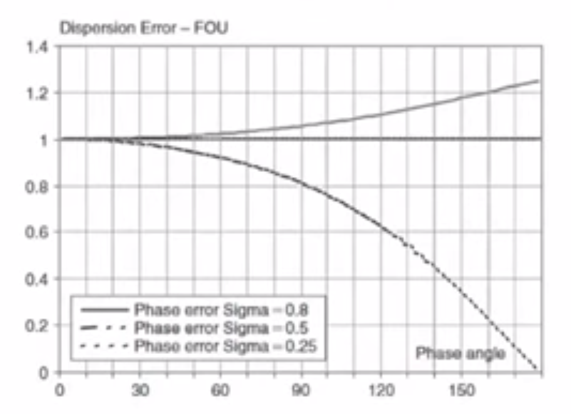
1.1.5.5.4.1. Dispersion (Phase) Error for 1st Order Upwind¶

For \(\sigma \gt 0.5 \Rightarrow \epsilon_\phi \gt 1 \Rightarrow\) Leading Error
For \(\sigma = 0.5 \Rightarrow \epsilon_\phi = 1 \Rightarrow\) No Error
For \(\sigma \lt 0.5 \Rightarrow \epsilon_\phi \lt 1 \Rightarrow\) Lagging Error

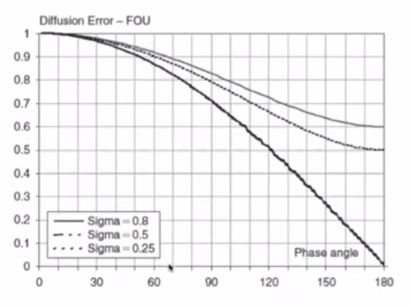
1.1.5.5.4.2. Diffusion (Amplitude) Error for 1st Order Upwind¶

Using \(\sigma = 0.5\) may give no dispersion error, but gives large diffusion error
The amplitude error increases dramatically with an increase in “frequency” i.e. reduced wavelength

Explanation of the Frequency Axis¶

Phase:

\[\phi = k \Delta x\]

Wavenumber:

\[k = {{2 \pi} \over \lambda}\]

So Phase i.t.o Wavenumber:

\[\phi = {{2 \pi} \over \lambda} \Delta x\]

Highest frequency you can represent in a mesh given by \(\lambda = 2 \Delta x \quad \Rightarrow \quad \phi = \pi\)

Test 1¶

\(k = 4 \pi\) and \(\phi = {\pi \over {12.5}}\)

Diffusion Error = 0.995

For 80 timesteps \(\left| G \right| ^n = (0.995)^{80} = 0.67\)

Test 2¶

\(\phi = {\pi \over {6.25}} = 28.8^{\circ}\)

For 80 timesteps \(\left| G \right| ^n = (0.98)^{80} = 0.20\)

This is a problem for first order schemes:

Only a small diffusion error (1%) for one timestep after 100 timesteps will lead to an amplitude error of 36%

1.1.5.5.5. Analysis of Lax-Friedrichs ¶

\[\left| G \right| = [cos^2 \phi + \sigma^2 sin^2 \phi]^{0.5}\]

\[\Phi = tan^{-1} (\sigma tan \phi)\]

Diffusion error:

\[\epsilon_D = [cos^2 \phi + \sigma^2 sin^2 \phi]^{0.5}\]

Dispersion error:

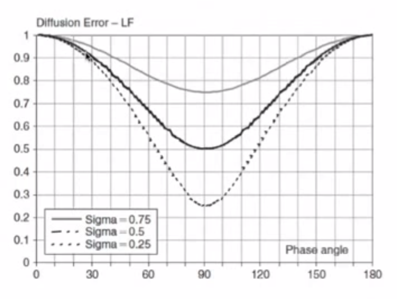
\[\epsilon_\Phi = {\Phi \over {\sigma \phi}} = { {tan^{-1} (\sigma tan \phi)} \over {\sigma \phi}}\]

1.1.5.5.5.1. Diffusion Error for Lax-Friedrichs¶

Amplitude strongly damped for small values of \(\sigma\)

No diffusion error for \(\phi = 0\) and \(\phi = \pi\)

\(\phi = \pi\) is related to the minimum realisable wavelength \(2 \Delta x\)

Any errors that occur at \(2 \Delta x\) will not be damped by the solution, which is related to the odd-even decoupling (the value of the point at i, n+1 doesn’t depend on the value at i, n)

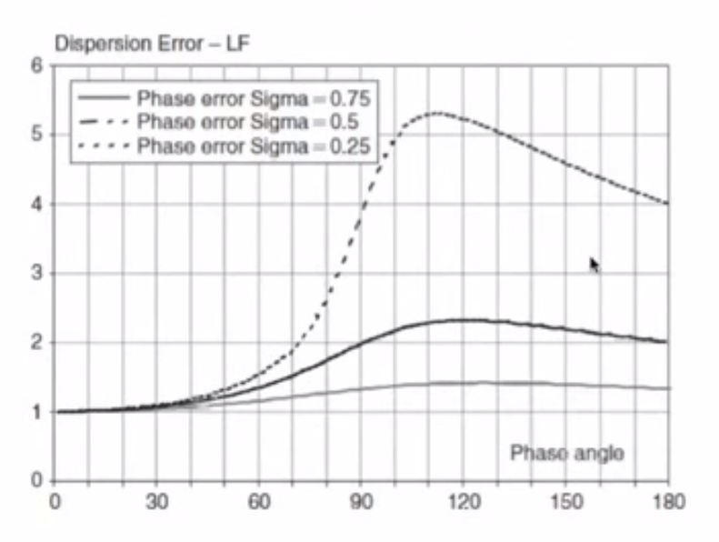
1.1.5.5.5.2. Dipersion Error for Lax-Friedrichs¶

Dispersion error \(\epsilon_{\Phi} \gt 1 \quad \Rightarrow \quad\) Leading Error

1.1.5.5.6. Analysis of Lax-Wendroff ¶

Dissipation error:

\[\left| G \right| = (1- 4 \sigma^2(1- \sigma^2)sin^4 {\phi \over 2})^{0.5}\]

Dispersion error:

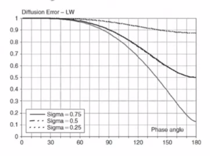
\[\epsilon_D = {{ {tan^{-1} [ (\sigma sin \phi) / (1-2 \sigma^2 sin^2 {\phi \over 2})]} \over {\sigma \phi}}}\]

1.1.5.5.6.1. Diffusion Error for Lax-Wendroff¶

Diffusion Error is close to one for a large phase range

Test 2¶

\(\phi = {\pi \over {6.25}} = 28.8^{\circ}\)

For \(sigma = 0.8 \qquad \epsilon_D = 0.9985\)

After 80 timesteps \(\left| G \right| ^n = (0.9985)^{80} = 0.89\)

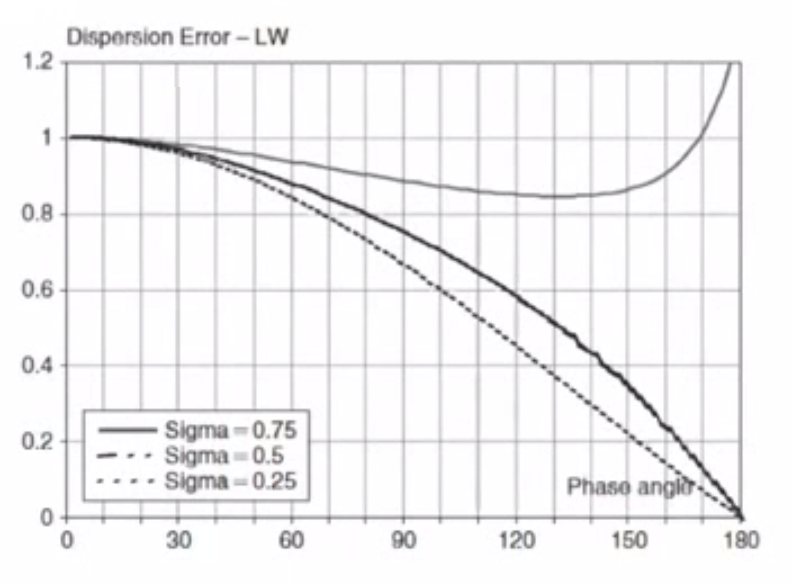
1.1.5.5.6.2. Dispersion Error for Lax-Wendroff¶

1.1.5.5.7. Summary ¶

1.1.5.5.7.1. Spectral Analysis¶

Error in amplitude or diffusion error:

\[\epsilon_D = {{\left| G \right|} \over {\left| \tilde{G} \right|}}\]

Error in the phase or dipsersion error:

\[\epsilon_{\phi} = {{\Phi} \over {\tilde{\Phi}}}\]

For a hyperbolic problem \(\left| \tilde{G} \right| = 1\)

\[\epsilon_{D} = {\left| G \right|}\]

\[\epsilon_{\phi} = {{c_{num}} \over c} = {{tan^{-1} {-Im (G) / Re (G)}} \over {\sigma \phi}}\]

Looked at plots of \(\epsilon_D\), \(\epsilon_{\phi}\) vs \(\phi ( = k \Delta x)\) with \(\sigma\) as parameter

1.1.5.5.7.2. 1st order Upwind¶

\(\epsilon_D\) decreases away from 1 quickly with increasing frequency. For high frequencies damping is very large - very difficult to use 1st order upwind for any transport problems

\(\epsilon_{\phi} \lt 1\) (lagging error - numerical convection velocity is slower than analytical) for \(\sigma \gt 0.5\)

\(\epsilon_{\phi} \gt 1\) (leading error) for \(\sigma \lt 0.5\)

\(\epsilon_{\phi} = 1\) (no error) for \(\sigma = 0.5\)

1.1.5.5.7.3. Lax-Friedrichs¶

Why? Introduced to stabilize FTCS

What? Introduced considerable numerical diffusion

\(\epsilon_D\) shows strong damping for smaller \(\sigma\) and no damping for \(\phi = \pi\) any errors that appear in the solution at twice the mesh size will not be damped - results in the staircase “jagged” result observed for the 1D Burgers Equation.

\(\epsilon_{\phi} \gt 1\) (leading error)

1.1.5.5.7.4. Lax-Wendroff¶

Second Order Method - little numerical diffusion
Oscillations appear in the solution - especially where the solution is non-smooth

\(\epsilon_D\) shows larger accurate region where \(\epsilon_D = 1\)

\(\epsilon_{\phi} \lt 1\) (lagging error)

1.1.5.5.8. Analysis of Leapfrog ¶

1.1.5.5.8.1. Diffusion Error¶

Note that \(\left| G \right| = 1 \quad \Rightarrow \quad\) No diffusion error

Leapfrog scheme is useful for simulations that are required for long-time simulations e.g. weather forecast codes

Can have stability problems with non-linear PDEs

1.1.5.5.8.2. Dispersion Error¶

\[\epsilon_D = \pm {{ {tan^{-1} [ (\sigma sin \phi) / \sqrt{(1-\sigma^2 sin^2 {\phi}})]} \over {\sigma \phi}}} = \pm {{sin^{-1}(\sigma sin \phi)} \over {\sigma \phi}}\]

\(\epsilon_{\phi} \lt 1\) (lagging error)

Accurate results for smooth solutions \(u(x)\) smooth:

Amplitudes correctly modelled
Low frequencies, the phase error is close to 1

Neutral stability \(\left| G \right| =1\) for all \(\sigma\) some problems, as high frequency errors are not damped

Leapfrog unstable for Burgers Equation. Not good for any high speed flows with shocks

1.1.5.5.9. What is the Origin of the Oscillations?¶

Have not explained the origin of oscillations

We can explain why they occur behind the travelling wave

Oscillations have high frequency
Dispersion error \(\epsilon_{\phi} \lt 1\) for LW and Leapfrog (especially at higher frequency) - Convection speed of errors is slower than the physical one
Leapfrog \(\epsilon_{\phi} \Rightarrow 0\) for \(\phi \Rightarrow \pi\) and so oscillations are stronger than for LW

1.1.5.5.10. Analysis of Beam-Warming ¶

Consider an alternative scheme due to Beam and Warming

1.1.5.5.10.1. Lax-Wendroff¶

Recalled derivation of LW for linear convection:

\[u_i^{i+1} = u_i^n - c \Delta t(u_x)_i + {{c^2 \Delta t^2} \over 2}(u_{xx})_i + O(\Delta t^3)\]

Lax Wendroff uses CD for the derivatives

1.1.5.5.10.2. Beam-Warming¶

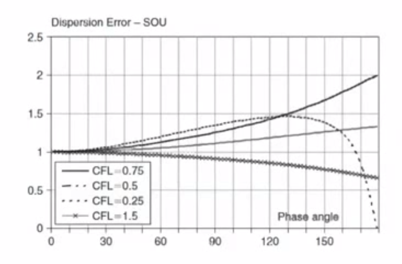
Beam-Warming uses 2nd order upwind for the derivatives

\[u_i^{i+1} = u_i^n - \sigma(3u_i^n - 4u_{i-1}^n+u_{i-2}^n) + {\sigma^2 \over 2}(u_i^n - 2u_{i-1}^n+u_{i-2}^n)\]

Diffusion Error¶

\[\left| G \right| = 1 - I \sigma [1 + 2(1- \sigma) sin^2 {\phi \over 2}]sin \phi- 2 \sigma [1 - (1- \sigma) cos \phi]sin^2{\phi \over 2}\]

Conditionally stable for \(0 \le \sigma \le 2\)

Diffusion error:

\[\epsilon_D = \left| G \right| = \sqrt{1 - \sigma(1-\sigma)^2(2-\sigma)(1-cos{\phi})^2}\]

Dispersion Error¶

\[\epsilon_{\phi} = \text{not given}\]

Beam-Warming shows flat region for a range of frequencies

Dispersion error \(\epsilon_{\phi} \gt 1\) for \(\sigma \lt 1\)

Numerical solution will move faster than analytical solution. High frequency oscillations should move ahead of the solution.

1.1.5.5.11. Final Notes ¶

1st order schemes generate large errors - not recommended
2nd order schemes acceptable errors - but should be careful with oscillations at higher frequencies

1.1.5.5.12. Implications of Diffusion Error for Grid Density ¶

Look at plot for \(\epsilon_D\) for LW, establishes a phase angle limit. We require \(\epsilon_D\) close to 1. Choose \(\phi_{lim} = 10^{\circ} = {\pi \over {18}}\) (arbitrarily).

Key quantity defining accuracy:

Number of mesh points per wavelength = \(N_{\lambda} = {\lambda \over {\Delta x}}\)
We require \(\phi = k \Delta x = {{2 \pi} \over \lambda} \le \phi_{lim}\)
Or:

\[N_{\lambda} = {\lambda \over {\Delta x}} \ge {{2 \pi} \over {\phi_{lim}}}\]

So if \(\phi_{lim} = {\pi \over {18}}\) then \(N_{lambda} = 36\) points per wavelength to resolve frequencies up to \({\pi \over {18}}\)

This is quite a severe requirement for unsteady problems

Even in steady problems you have artificial time in a transient period - otherwise you have an excessively damped solution.

1.1.5.5.13. Question ¶

What is the dissipation error for \(\sigma = 1\) ? For upwind is this a horizontal line?