1.1.5.3. The Diffusion of Heaviside and Sinusoidal Input
1.1.5.3.1. New Schemes for Linear Convection
Lax-Friedrichs \(\Rightarrow\) stabilizes CD, 1st order
Lax-Wendroff \(\Rightarrow\) stable CD with an additional dissipative term, 2nd order
Leapfrod \(\Rightarrow\) 2nd order, 3 level scheme (it is not self-starting)
1.1.5.3.2. Heaviside Function Input
The Heaviside Function represents a shock wave in velocity and pressure for compressible flow. One of the great challenges in numerical methods is representing sharp gradients.
The Wave Equation for these tests is described as follows:
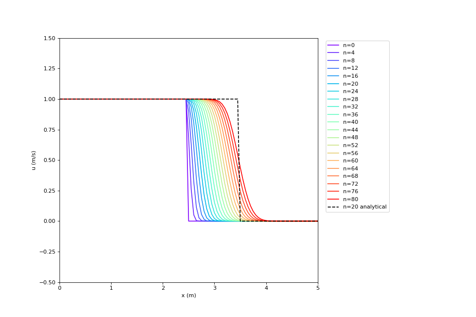
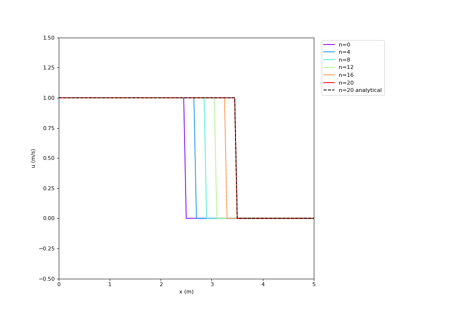
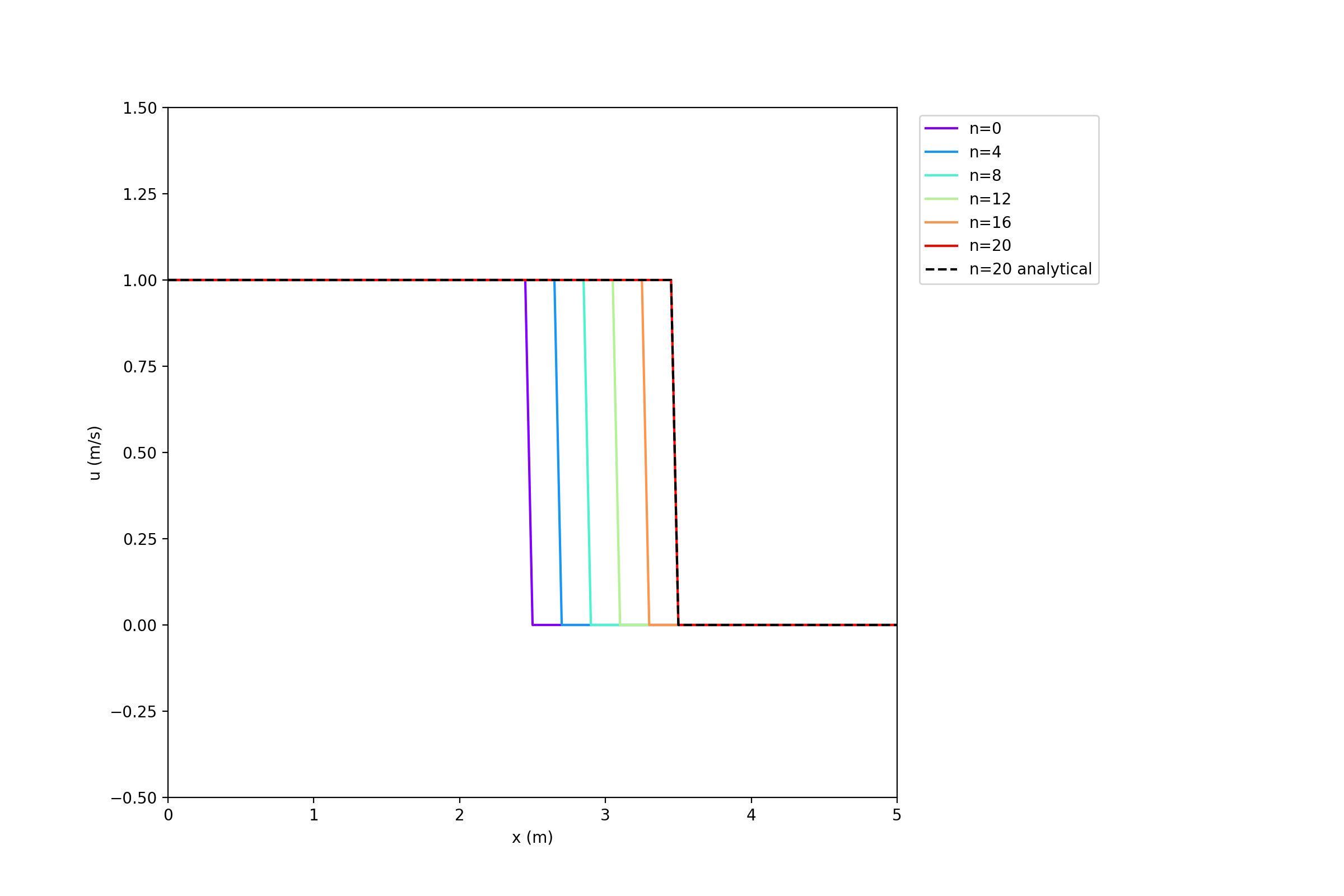
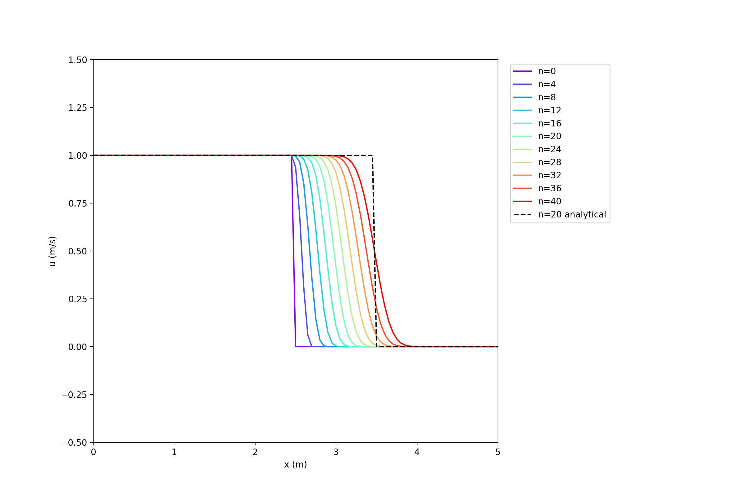
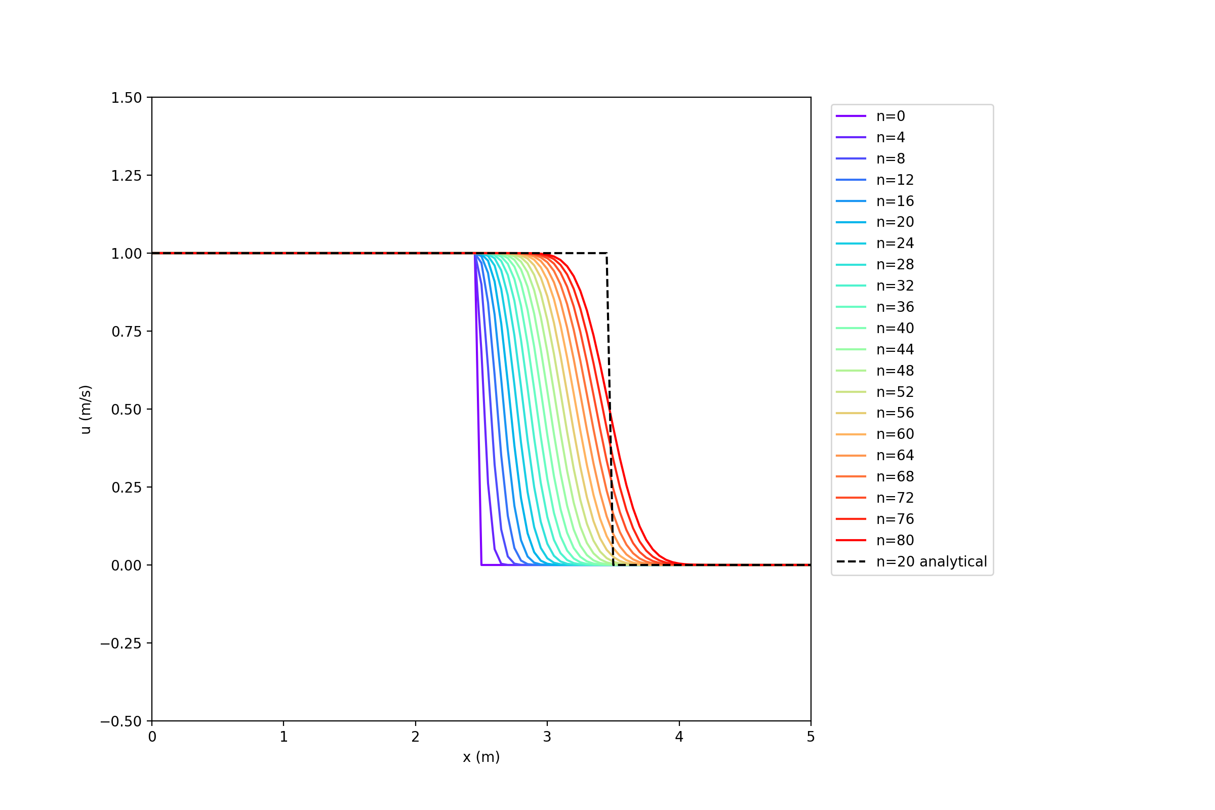
1.1.5.3.2.1. Upwind Differencing with \(\sigma = 1\), \(\sigma = 0.5\) and \(\sigma = 0.25\)
\(\sigma = 1\)
If the value of \(\sigma = 1\) then the new velocity simply equals the old velocity.
The phase angle is zero, so there is no diffusion or dispersion error
\(\sigma = 0.5\)
The jump is diffused by the numerical diffusion arising from the first order truncation error
The amount of diffusion is increasing as we move through time (as n increases)
The numerical speed with which the solution moves through the domain is also reduced
\(\sigma = 0.25\)
Clearly, the smaller Courant Number reduces the speed at which the solution travels through the domain
At these very low frequencies, there is not much more added diffusion between \(\sigma = 0.50\) and \(\sigma = 0.25\)


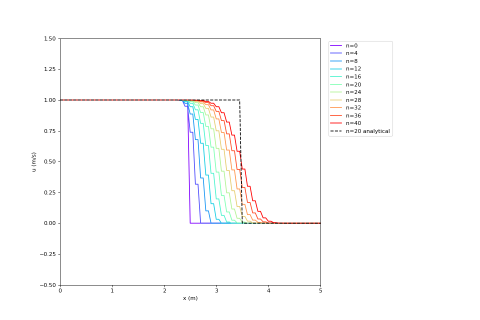
1.1.5.3.2.2. Lax-Friedrichs with \(\sigma = 0.5\)
Numerical dissipation (more than upwind scheme) and odd-even decoupling
Amount of diffusion is still increasing with increasing n

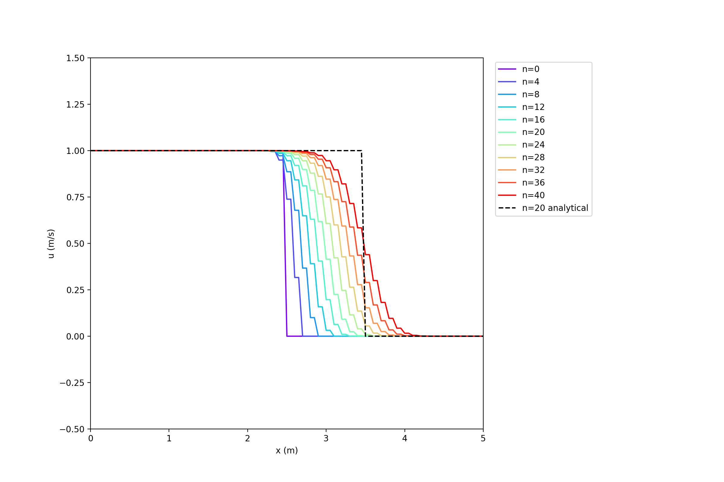
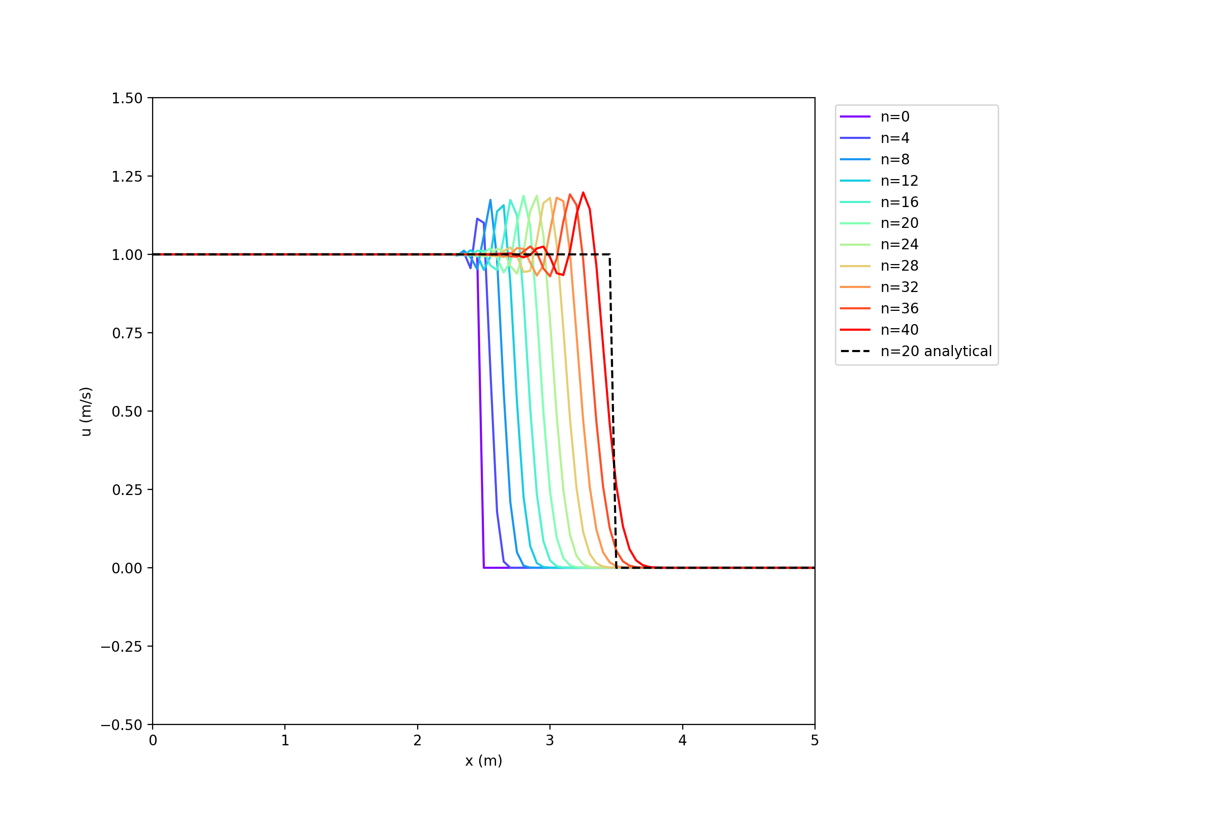
1.1.5.3.2.3. Lax-Wendroff with \(\sigma = 0.5\)
This more accurately represents the step change
However, there is an oscillatory response
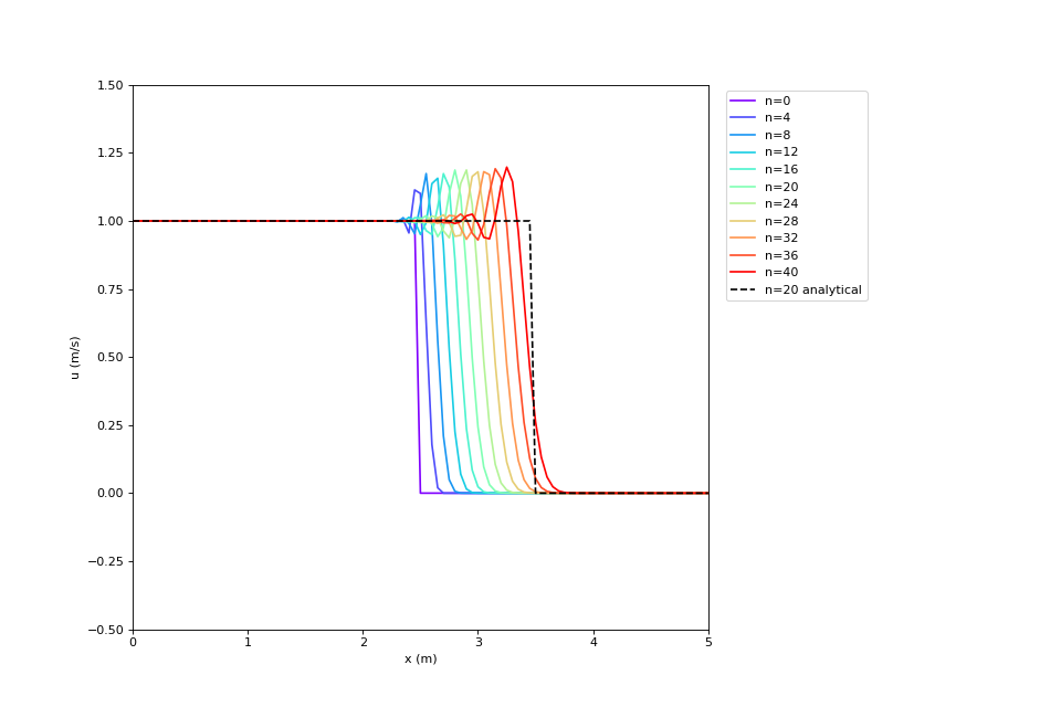
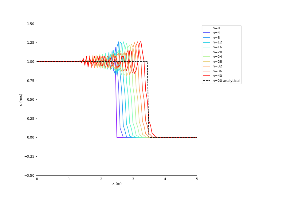
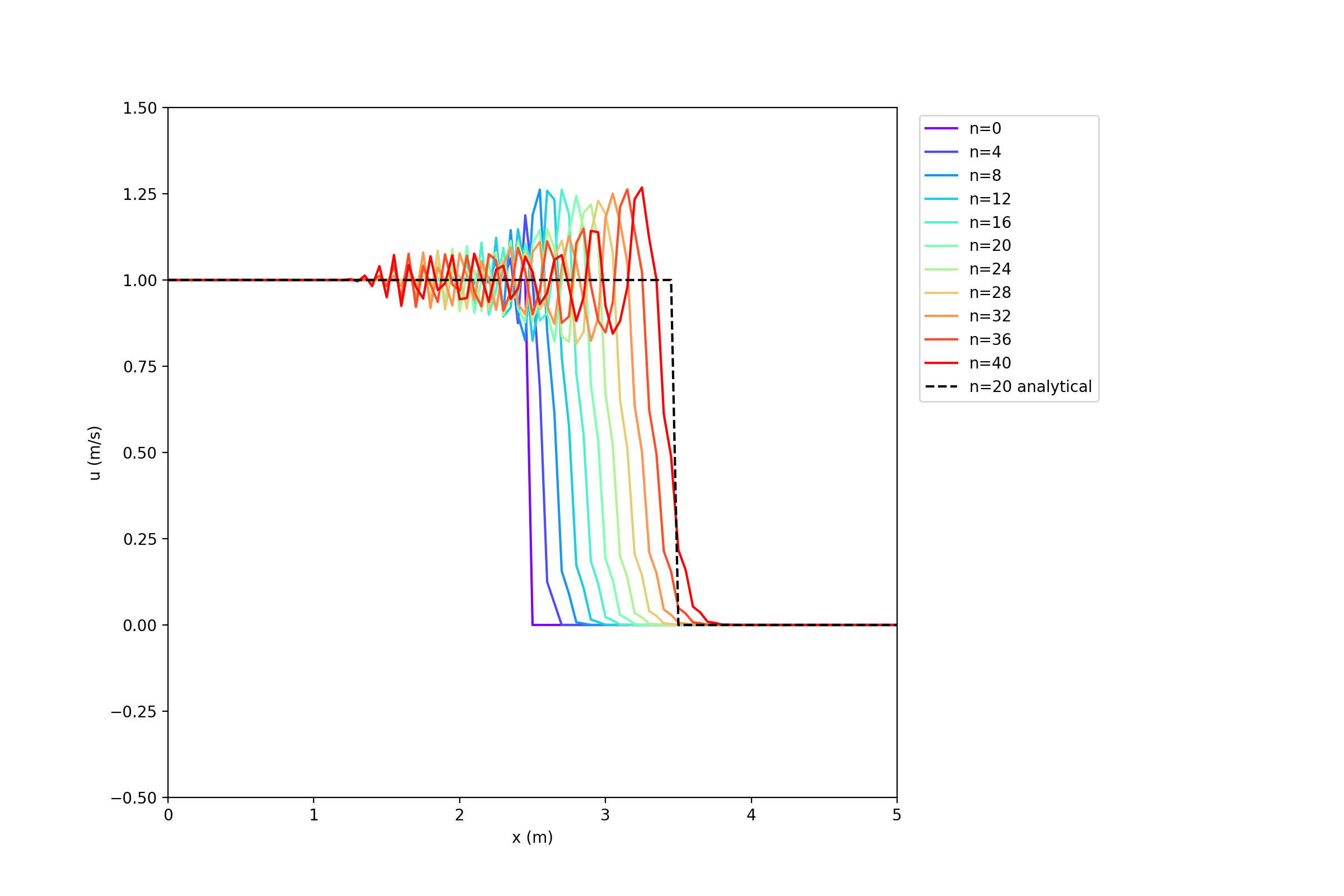
1.1.5.3.2.4. Leapfrog with \(\sigma = 0.5\)
More oscillatory than Lax-Wendroff, more accurate than Lax-Friedrichs

1.1.5.3.2.5. Results of Test 1: Heaviside Function
Why does Lax-Friedrichs show step changes in the output?
This is a double solution effect:
\(u_i^{n+1}\) does not depend on \(u_i^n\)
Shifting the stencil by \(i\) shows that \(u_i^{n+1}\) and \(u_{i+1}^{n+1}\) do not share a single mesh point of their stencils
This is called “odd-even decoupling”
Odd-Even Decoupling: * Solutions on the odd points and even points have different error levels and can’t communicate information * One solution sightly ahead/slightly behind

Why does Lax-Wendroff show good comparison with the analytical solution?
Lax-Wendroff is second order, so has reduced numerical diffusion
However, numerical oscillations occur. More oscillations occur with Leapfrog than Lax-Wendroff
1.1.5.3.3. Sinusoidal Input, \(k = 4 \pi\)
Travelling sinusoidal wave, 2 periods in a distance of 1m. Corresponding wave number:
This is the initial condition.
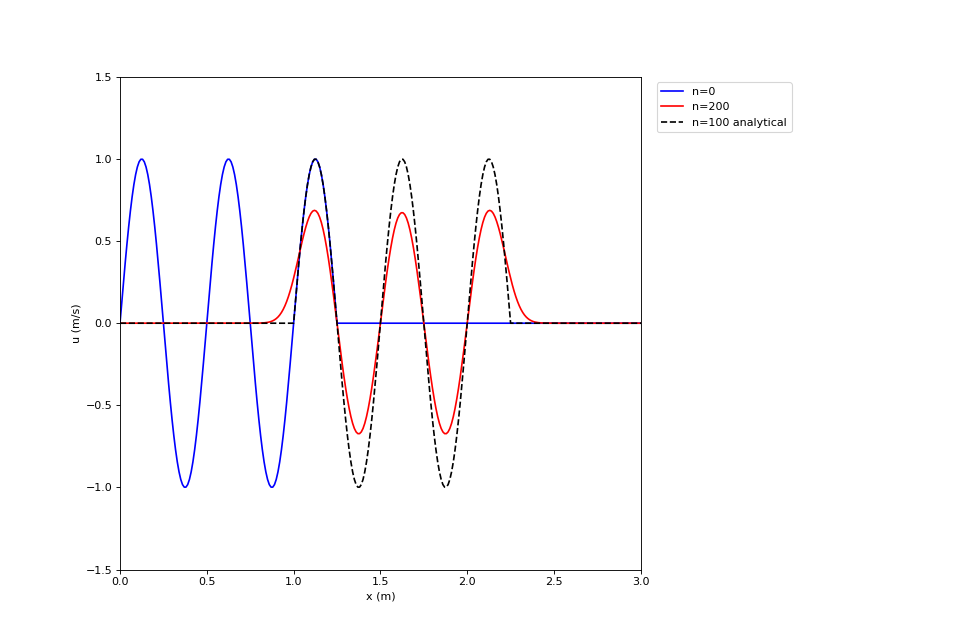
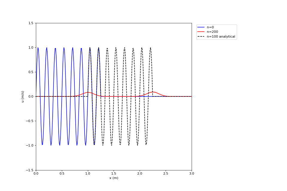
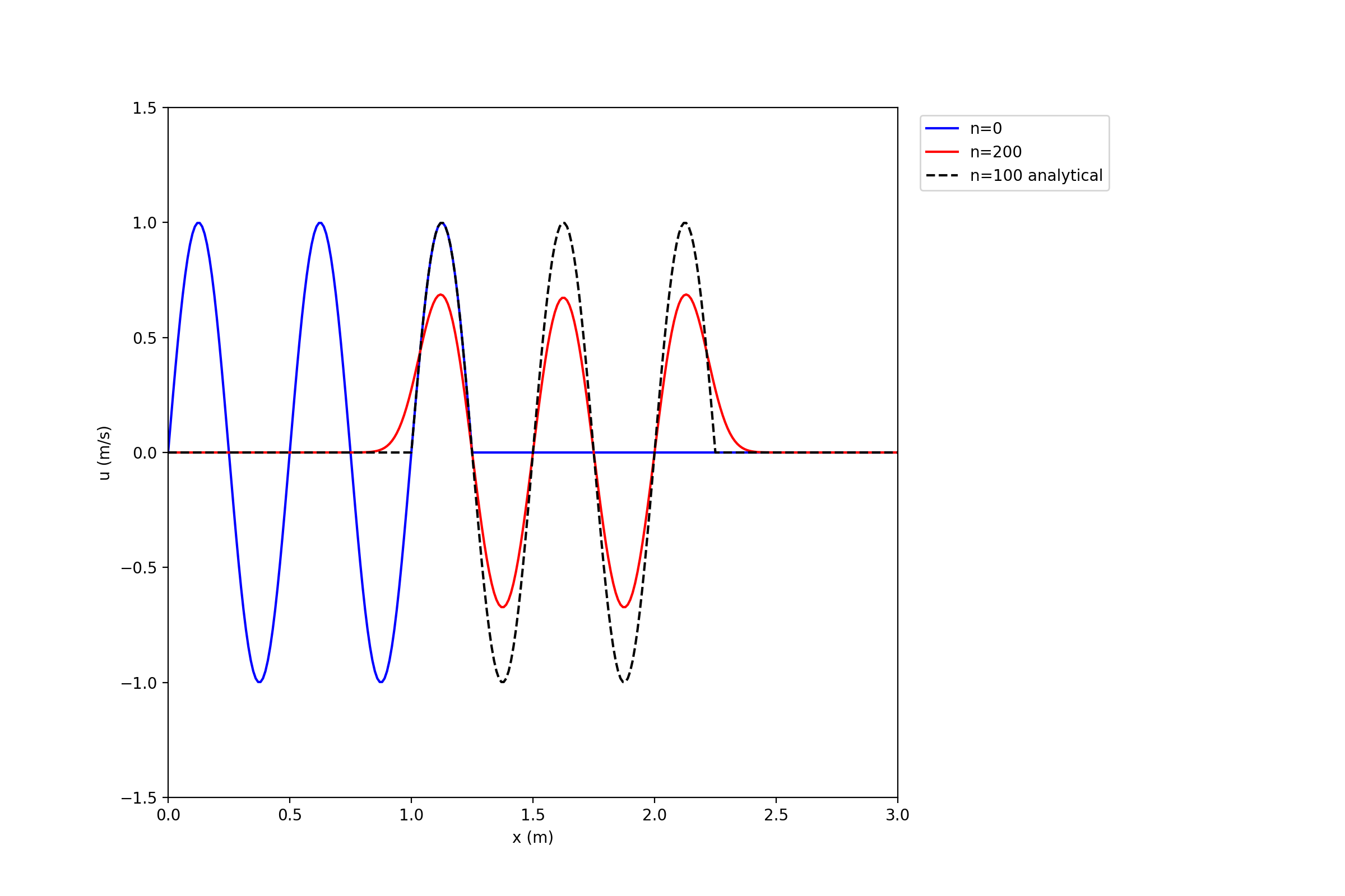
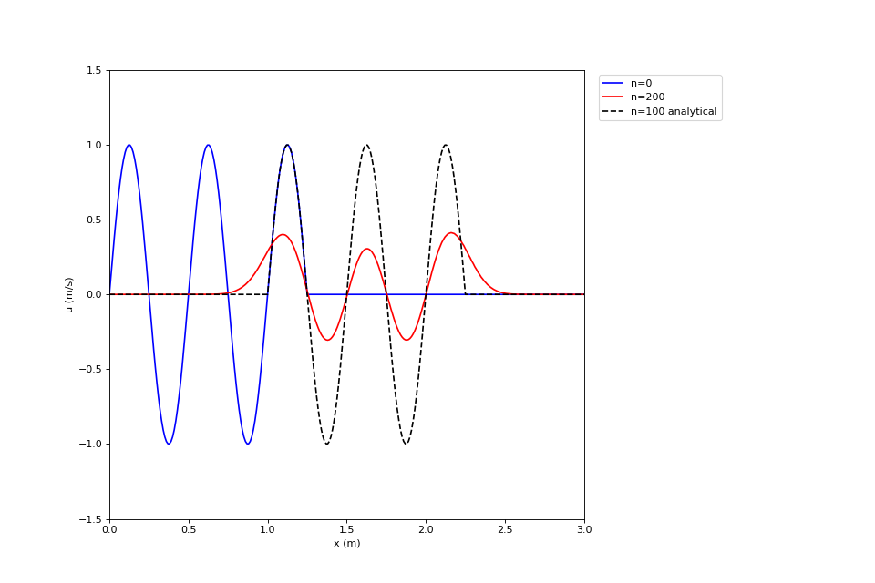
1.1.5.3.3.1. Upwind Differencing with \(\sigma = 0.5\)
Amplitude is being diffused, effective numerical diffusion after a number of timesteps
Damped by backward difference method

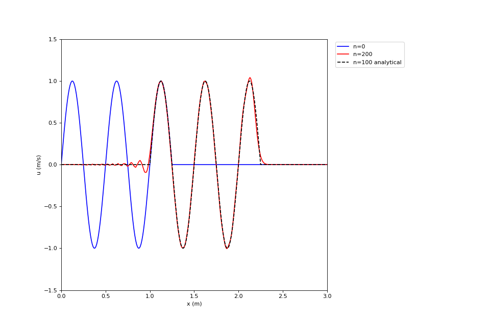
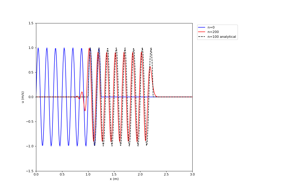
1.1.5.3.3.3. Lax-Wendroff with \(\sigma = 0.5\)
Better representation of the wave
Wiggles at the back of the wave, where there is a non-smooth slope

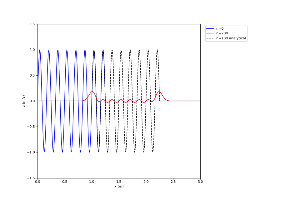
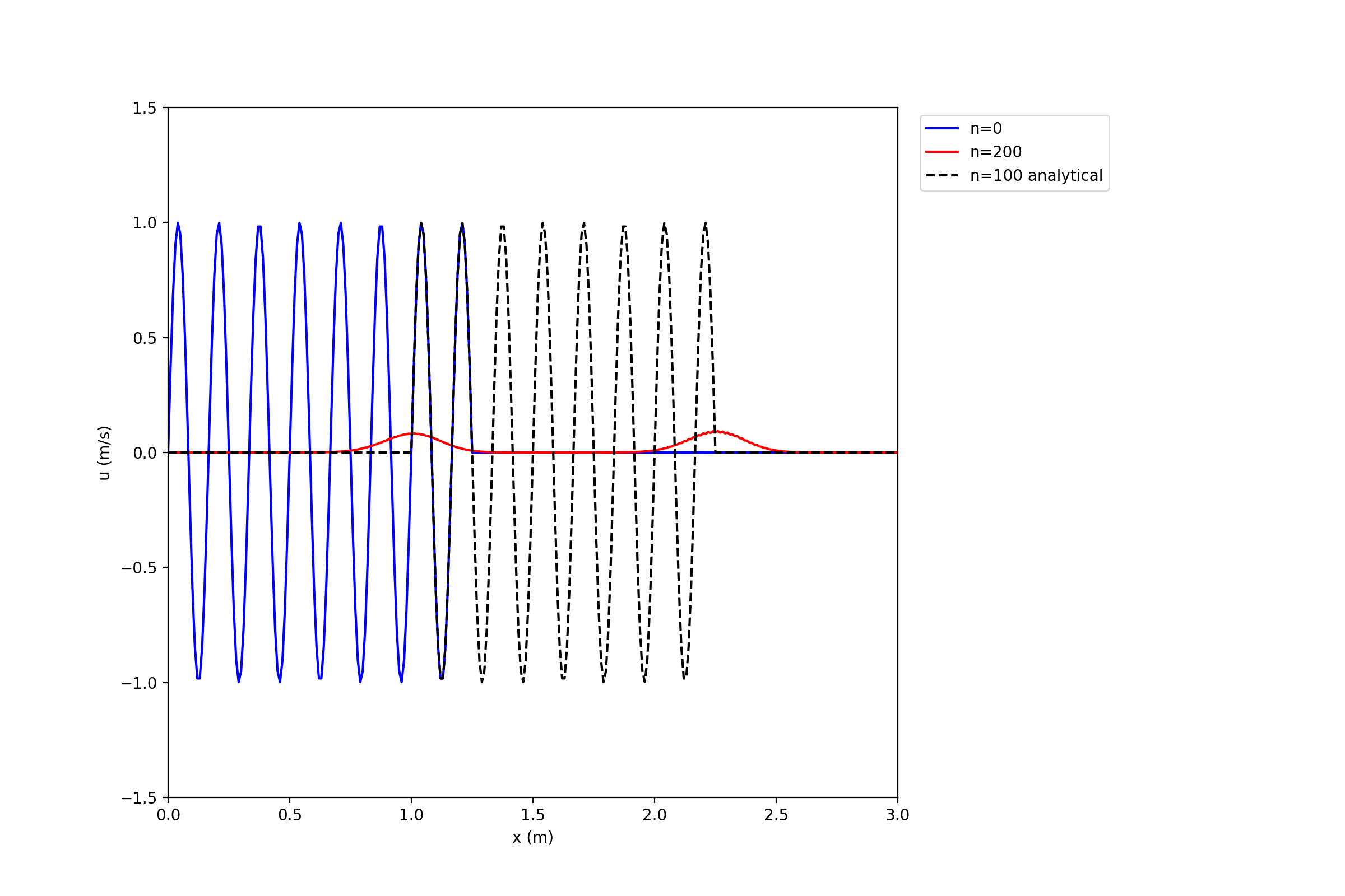
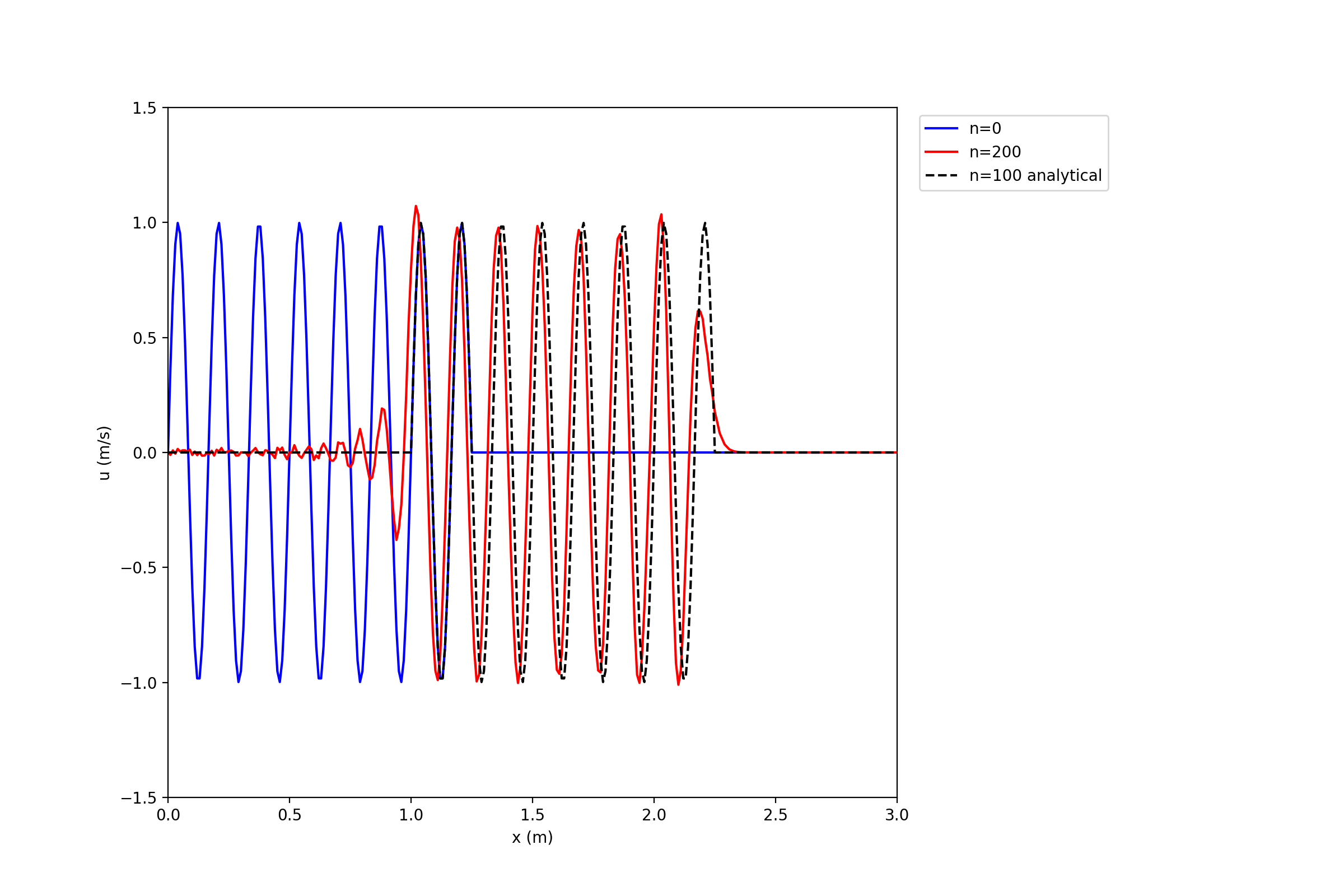
1.1.5.3.4. Sinusoidal Input, \(k = 10 \pi\)
Travelling sinusoidal wave. Corresponding wave number:
This is the initial condition.


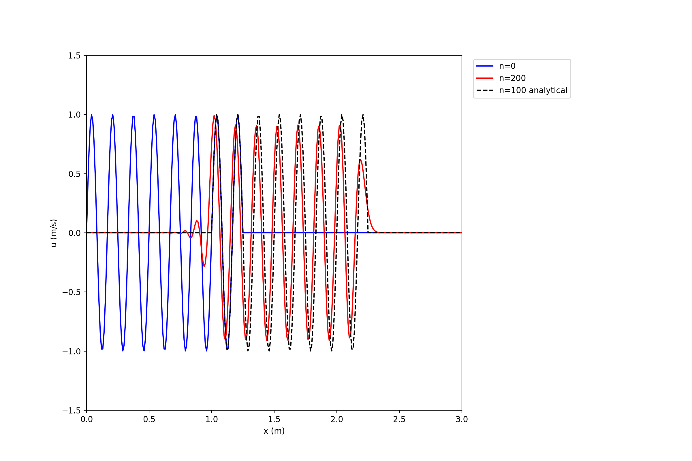
1.1.5.3.4.5. Results of Test 3: High Frequency Sinusoidal Input
Implications
Upwind and Lax Friedrichs are catastrophically dissipative
Lax Wendroff shows some dissipation and a lag
Leapfrog shows less dissipation, but more oscillations and still a lag
1.1.5.3.5. Summary
1st order schemes:
Have poor accuracy - gets even worse for solutions with higher frequency, damping is catastrophic
2nd order schemes:
Provide better accuracy
Generate numerical oscillations - associated with locations where solution is not smooth. Oscillations are stronger with Leapfrog scheme
Numerical errors are sensitive to the frequency content of the solution, i.e frequency content of initial condition
We have obtained results from simple 1D models, however they are representative of real flow situations (2D, 3D etc)