6. Examples of the Finite Volume Method with Numerical Methods¶

2D Diffusion Equation
Lax-Wendroff Method in FVM
MacCormack Method in FVM
- Cell-Centered Formulation
- Boundaries

6.1. 2D Diffusion Equation ¶

For example - 2D diffusion equation:

\[{\partial u \over \partial t} + {\partial \over \partial x} \left( k {\partial u \over \partial x} \right) + {\partial \over \partial y} \left( k {\partial u \over \partial y} \right) = 0\]

Diffusive Flux:

\[f = k {\partial u \over \partial x}\]

\[g = k {\partial u \over \partial y}\]

Balance of fluxes:

To express the balance of fluxes, we use

\[f_{AB} = {1 \over 2}(f_A + f_B)\]

We can’t evaluate \(f_{AB}\) perpendicular to the face, because we’d need values at the midpoints. The gradient evaluation is on the basis of Gauss’ Divergence Theorem, which requires a line integral over a 4 neighbour surfaces, where the corners are points we know the values of.

To get \(f_A\) and \(f_B\) we need to evalutate \(\partial u / \partial x\):

\[f_A = k \left( \partial \overline{u} \over \partial x \right)_A\]

6.2. Lax-Wendroff Method in FVM ¶

Recall for the model equation:

\[{\partial u \over \partial t} + {\partial \over \partial x} f(u)\]

We used the Taylor Expansion:

\[u^{n+1} = u^n + \Delta t \left( {\partial u \over \partial t} \right)^n + {{\Delta t^2} \over 2} \left(\partial ^2 u \over \partial t^2 \right)^n\]

And we use:

\[u_{tt} = (u_t)_t = - {\partial \over \partial t} \left(\partial f \over \partial x \right) = - {\partial \over \partial x} \left(\partial f \over \partial t \right) = - {\partial \over \partial x} \left({\partial f \over \partial u} {\partial u \over \partial t} \right) = {\partial \over \partial x} \left(a(u) {\partial f \over \partial x} \right)\]

where:

\(a = {\partial f \over \partial u}\) is the Jacobian

(1)\[u^{n+1} = u^n + \Delta t \left( -{\partial f \over \partial x} \right)^n + {{\Delta t^2} \over 2} \left({\partial \over \partial x} \left( {a {\partial f \over \partial x}} \right) \right)^n\]

2D version:

(2)\[\mathbf{u}^{n+1} = \mathbf{u}^n + \Delta t \left( -{\partial f \over \partial x} - {\partial g \over \partial y} \right)^n + {{\Delta t^2} \over 2} \left( {\partial \over \partial x} \left( {A^n \left( {\partial f \over \partial x} + {\partial g \over \partial y} \right)^n } \right)+ {\partial \over \partial y} \left( {B^n \left( {\partial f \over \partial x} + {\partial g \over \partial y} \right)^n } \right) \right)\]

\(A = {\partial f \over \partial u}\) and \(B = {\partial g \over \partial u}\)

(1) and (2) can be discretised using the FDM to get one step LW

Note that they have the form of a flux balance - in theory can use FVM - however the fluxes contain derivatives

For this reason, one-step LW is not used with the finite volume.

Instead, we can use MacCormack

6.3. MacCormack Method in FVM ¶

Write (1) in MacCormack:

Predictor:

\[\tilde{u}_i^{n+1} = u_i^n - {\Delta t \over \Delta x} (f_{i+1}^n - f_i^n)\]

Corrector:

\[u_i^{n+1} = {1 \over 2}(u_i^n + \tilde{u}_i^{n+1}) - {\Delta t \over {2 \Delta x}} (\tilde{f}_i^{n+1} - \tilde{f}_{i-1}^{n+1})\]

FV formulation: mimic “forward-backward” predictor-corrector approach in flux evaluation

6.3.1. Cell-Centered Formulation ¶

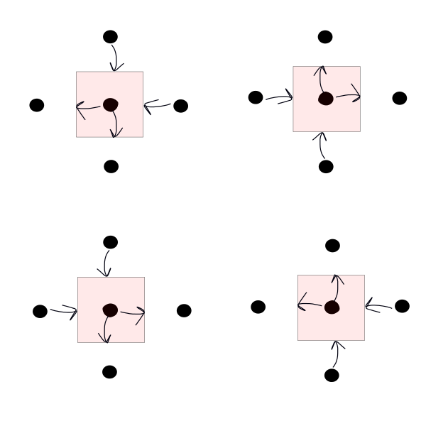
Possible variants for the predictor step. Invert bias for the corrector step. 4 choices:

6.3.2. Boundaries ¶

Inflow/outflow - extrapolation formulas are used
Solid boundaries - convective fluxes are set to zero

The Visual Room