1. Multi-step Numerical Methods
Summary:
- Schemes presented for linear equations are not well-suited to the solution of non-linear problems
- Multi-step methods work well in non-linear hyperbolic equations
- FD schemes at split time levels, also called “predictor-corrector” methods
- Richtmyer/Lax-Wendroff
- MacCormack
1.1. About Multi-step methods
Multi-step are FD schemes are at split time levels and work well in non-linear hyperbolic problems. They are also called predictor-corrector methods.
- 1st step, a “temporary value” for u(x) is “predicted”
- 2nd step a “corrected value” is computed
1.2. Richtmyer/Lax-Wendroff
Two variants:
- Variant 1 - Richtmyer - at point \(i\)
- Variant 2 - 2 step LW - at point \(i + {1 \over 2}\)
1.2.1. Variant 1 - Richtmyer (Lax-Friedrichs and Leapfrog)
- Step 1: Predictor Step use LF method at time level \(n + {1 \over 2}\)
\[{{u_i^{n+{1 \over 2}} - {1 \over 2} (u_{i+1}^n + u_{i-1}^n)} \over {{\Delta t} \over 2 } }
=-c{ {( {u_{i+1}^n - u_{i-1}^n})} \over {2 \Delta x}}\]
- Step 2: Corrector Step Leapfrog with \({\Delta t} \over 2\)
\[{{u_i^{n+1} - u_i^n} \over {\Delta t} }
=-c{ {( {u_{i+1}^{n+{1 \over 2}} - u_{i-1}^{n+{1 \over 2}}})} \over {2 \Delta x}}\]
Transpose Step 1 and 2 for outputs:
- Predictor:
\[u_i^{n+{1 \over 2}} = {1 \over 2} (u_{i+1}^n + u_{i-1}^n) - {\sigma \over 4}(u_{i+1}^n - u_{i-1}^n)\]
- Corrector:
\[u_i^{n+1} = u_i^{n-1} - {\sigma \over 2} (u_{i+1}^{n+{1 \over 2}} - u_{i-1}^{n+{1 \over 2}})\]
- Stable for Courant Number = \(\sigma = {{c \Delta t} \over {\Delta x}} \le 2\) (possibly as a consequence of the half-time step in the method?)
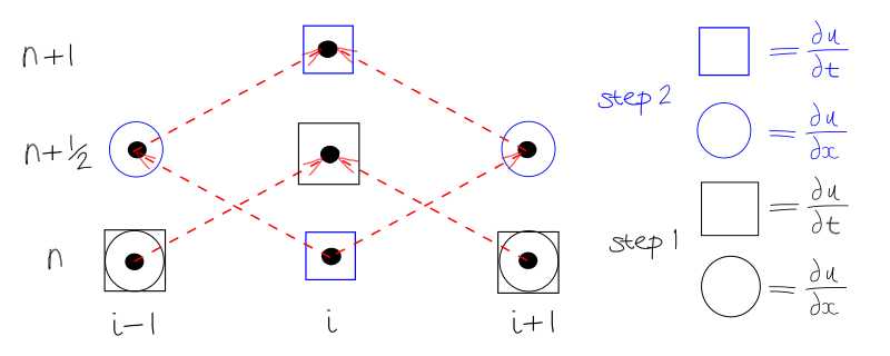
1.2.2. Variant 2 - 2 Step Lax-Wendroff
- Step 1: Predictor Step use LF on \(i+{1 \over 2}\)
\[u_{i+{1 \over 2}}^{n+{1 \over 2}} = {1 \over 2} (u_{i+1}^n + u_{i}^n) - {\sigma \over 2}(u_{i+1}^n - u_{i}^n)\]
- Step 2: Corrector Step use FTCS
\[u_i^{n+1} = u_i^{n} - {\sigma} (u_{i+{1 \over 2}}^{n+{1 \over 2}} - u_{i-{1 \over 2}}^{n+{1 \over 2}})\]
- Stable for Courant Number = \(\sigma = {{c \Delta t} \over {\Delta x}} \le 1\)

- This scheme is 2nd order
- For linear PDEs it is equivalent to the single step LW
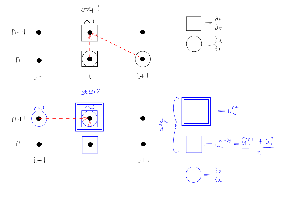
1.3. MacCormack Method
- Step 1 - uses FD scheme in x - call \(\tilde{u}^{n+1}\) the temporary solution
\[{{\tilde{u}_i^{n+1} - u_i^n} \over {\Delta t}} = -c {{{(u_{i+1}^n - u_i^n)}} \over {\Delta x}}\]
- Step 2 - uses BD scheme in x with \({{\Delta t} \over 2}\)
\[{{u_i^{n+1} - u_i^{n+{1 \over 2}} } \over {{\Delta t} \over 2}}
= -c{{({\tilde{u}_{i}^{n+1} - \tilde{u}_{i-1}^{n+1}})} \over {\Delta x}}\]
and replace the value \(u_i^{n+{1 \over 2}}\) by the average
\[{u_i^{n + {1 \over 2}}} = {1 \over 2}(u_i^n + \tilde{u}_i^{n+1})\]
- Predictor
\[\tilde{u}_i^{n+1} = u_i^n - {{c \Delta t} \over {\Delta x}} (u_{i+1}^n - u_i^n)\]
- Corrector
\[u_i^{n+1} = {1 \over 2} \left [ (u_i^n + \tilde{u}_i^{n+1}) - {{c \Delta t} \over {\Delta x}} (\tilde{u}_i^{n+1} - \tilde{u}_{i-1}^{n+1}) \right ]\]
- 2nd order method
- Stability \(\sigma < 1\)
- For linear PDEs equivalent to LW
- Can alternate FD/BD - BD/FD works well for nonlinear problems
- Don’t need to store values at intermediate mesh points (like 2 step Lax Wendroff)
1.4. Conclusion
- The majority of PDEs in fluid mechanics are non-linear
- You can learn a lot by just studying Burgers Equation, that are especially important if you are studying the Euler Equations (for compressible flows)
- In general, the non-linearity dominates over viscous terms - especially in high Reynolds Number flows - but not for mixing flows, e.g. Stokes flow (where viscous terms dominate)
- So studying inviscid Burgers equation has important consequences for fluid mechanics