7. 2D Second-order Linear Diffusion
7.1. Understand the Problem
- What is the final velocity profile for 2D linear diffusion when the initial conditions are a square wave and the boundary conditions are unity?
- 2D diffusion is described as follows:
\[{\partial u \over \partial t} = \nu \left ( {\partial^2 u \over \partial x^2}+ {\partial^2 u \over \partial y^2} \right )\]
\[{\partial v \over \partial t} = \nu \left ( {\partial^2 v \over \partial x^2}+ {\partial^2 v \over \partial y^2} \right )\]
7.2. Formulate the Problem
7.2.1. Input Data
- nt = 51 (number of temporal points)
- tmax = 0.5
- nx = 21 (number of x spatial points)
- nj = 21 (number of y spatial points)
- xmax = 2
- ymax = 2
- nu = 0.1
Initial Conditions: \(t=0\)
| x | i | y | j | u(x,y,t), v(x,y,t) |
|---|---|---|---|---|
| \(0\) | \(0\) | \(0\) | \(0\) | \(1\) |
| \(0 < x \le 0.5\) | \(0 < i \le 5\) | \(0 < y \le 0.5\) | \(0 < j \le 5\) | \(1\) |
| \(0.5 < x \le 1\) | \(5 < i \le 10\) | \(0.5 < y \le 1\) | \(5 < j \le 10\) | \(2\) |
| \(1 < x < 2\) | \(10 < i < 20\) | \(1 < y < 2\) | \(10 < j < 20\) | \(1\) |
| \(2\) | \(20\) | \(2\) | \(20\) | \(1\) |
Boundary Conditions: \(x=0\) and \(x=2\), \(y=0\) and \(y=2\)
| t | n | u(x,y,t), v(x,y,t) |
|---|---|---|
| \(0 \le t \le 0.5\) | \(0 \le n \le 50\) | \(1\) |
7.2.2. Output Data
| x | y | t | u(x,y,t), v(x,y,t) |
|---|---|---|---|
| \(0 \le x \le 2\) | \(0 \le y \le 2\) | \(0 \le t \le 0.5\) | \(?\) |
7.3. Design Algorithm to Solve Problem
7.3.1. Space-time discretisation
- i \(\rightarrow\) index of grid in x
- j \(\rightarrow\) index of grid in y
- n \(\rightarrow\) index of grid in t
7.3.2. Numerical scheme
- FD in time
- CD in space
7.3.3. Discrete equation
\[{{u_{i,j}^{n+1} - u_{i,j}^n} \over {\Delta t}} =
\nu {{u_{i-1,j}^n - 2u_{i,j}^n + u_{i+1,j}^n} \over \Delta x^2} +
\nu {{u_{i,j-1}^n - 2u_{i,j}^n + u_{i,j+1}^n} \over \Delta y^2}\]
\[{{v_{i,j}^{n+1} - v_{i,j}^n} \over {\Delta t}} =
\nu {{v_{i-1,j}^n - 2v_{i,j}^n + v_{i+1,j}^n} \over \Delta x^2} +
\nu {{v_{i,j-1}^n - 2v_{i,j}^n + v_{i,j+1}^n} \over \Delta y^2}\]
7.3.4. Transpose
\[u_{i,j}^{n+1} =
u_{i,j}^n +
\nu \Delta t \left ( {{u_{i-1,j}^n - 2u_{i,j}^n + u_{i+1,j}^n} \over \Delta x^2} +
{{u_{i,j-1}^n - 2u_{i,j}^n + u_{i,j+1}^n} \over \Delta y^2} \right )\]
\[v_{i,j}^{n+1} =
v_{i,j}^n +
\nu \Delta t \left ( {{v_{i-1,j}^n - 2v_{i,j}^n + v_{i+1,j}^n} \over \Delta x^2} +
{{v_{i,j-1}^n - 2v_{i,j}^n + v_{i,j+1}^n} \over \Delta y^2} \right )\]
7.3.5. Pseudo-code
#Constants
nt = 51
tmax = 0.5
dt =  tmax/(nt-1)
nx =  21
xmax = 2
ny = 21
ymax = 2
dx = xmax/(nx-1)
dy = ymax/(ny-1)
nu = 0.1

#Boundary Conditions
#u boundary, bottom and top
u(0:20,0,0:50)=u(0:20,20,0:50)=1
#v boundary, bottom and top
v(0:20,0,0:50)=v(0:20,20,0:50)=1
#u boundary left and right
u(0,0:20,0:50)=u(20,0:20,0:50)=1
#v boundary left and right
v(0,0:20,0:50)=v(20,0:20,0:50)=1

#Initial Conditions
u(:,:,0) = 1
v(:,:,0) = 1
u(5:10,5:10,0) = 2
v(5:10,5:10,0) = 2

#Iteration
for n between 0 and 49
   for i between 1 and 19
      for j between 1 and 19
          u(i,j,n+1) = u(i,j,n)-dt*nu*[ ( u(i-1,j,n)-2*u(i,j,n)+u(i+1,j,n) ) /dx^2 +
                                        ( u(i,j-1,n)-2*u(i,j,n)+u(i,j+1,n) ) /dy^2 ]
          v(i,j,n+1) = v(i,j,n)-dt*nu*[ ( v(i-1,j,n)-2*v(i,j,n)+v(i+1,j,n) ) /dx^2 +
                                        ( v(i,j-1,n)-2*v(i,j,n)+v(i,j+1,n) ) /dy^2 ]
7.4. Implement Algorithm in Python
def diffusion(nt, nx, ny, tmax, xmax, ymax, nu):
   """
   Returns the velocity field and distance for 2D diffusion
   """
   # Increments
   dt = tmax/(nt-1)
   dx = xmax/(nx-1)
   dy = ymax/(ny-1)

   # Initialise data structures
   import numpy as np
   u = np.zeros(((nx,ny,nt)))
   v = np.zeros(((nx,ny,nt)))
   x = np.zeros(nx)
   y = np.zeros(ny)

   # Boundary conditions
   u[0,:,:] = u[nx-1,:,:] = u[:,0,:] = u[:,ny-1,:] = 1
   v[0,:,:] = v[nx-1,:,:] = v[:,0,:] = v[:,ny-1,:] = 1

   # Initial conditions
   u[:,:,:] = v[:,:,:] = 1
   u[(nx-1)/4:(nx-1)/2,(ny-1)/4:(ny-1)/2,0] = 2
   v[(nx-1)/4:(nx-1)/2,(ny-1)/4:(ny-1)/2,0] = 2

   # Loop
   for n in range(0,nt-1):
      for i in range(1,nx-1):
         for j in range(1,ny-1):
            u[i,j,n+1] = ( u[i,j,n]+dt*nu*( ( u[i-1,j,n]-2*u[i,j,n]+u[i+1,j,n] ) /dx**2 +
                                          ( u[i,j-1,n]-2*u[i,j,n]+u[i,j+1,n] ) /dy**2 ) )
            v[i,j,n+1] = ( v[i,j,n]+dt*nu*( ( v[i-1,j,n]-2*v[i,j,n]+v[i+1,j,n] ) /dx**2 +
                                          ( v[i,j-1,n]-2*v[i,j,n]+v[i,j+1,n] ) /dy**2 ) )

   # X Loop
   for i in range(0,nx):
      x[i] = i*dx

   # Y Loop
   for j in range(0,ny):
      y[j] = j*dy

   return u, v, x, y

def plot_3D(u,x,y,time,title,label):
   """
   Plots the 2D velocity field
   """

   import matplotlib.pyplot as plt
   from mpl_toolkits.mplot3d import Axes3D
   fig=plt.figure(figsize=(11,7),dpi=100)
   ax=fig.gca(projection='3d')
   ax.set_xlabel('x (m)')
   ax.set_ylabel('y (m)')
   ax.set_zlabel(label)
   X,Y=np.meshgrid(x,y)
   surf=ax.plot_surface(X,Y,u[:,:,time],rstride=2,cstride=2)
   plt.title(title)
   plt.show()
u,v,x,y = diffusion(151, 51, 51, 0.5, 2.0, 2.0, 0.1)
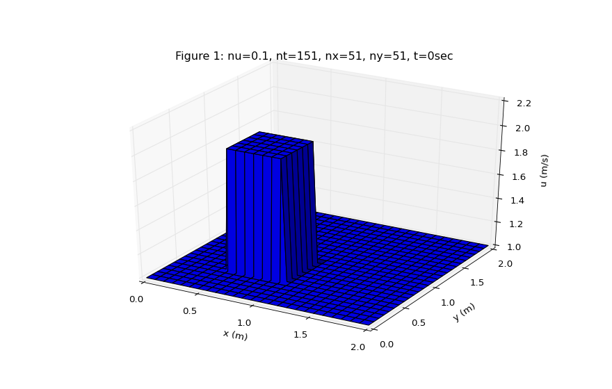
plot_3D(u,x,y,0,'Figure 1: nu=0.1, nt=151, nx=51, ny=51, t=0sec','u (m/s)')
plot_3D(u,x,y,100,'Figure 2: nu=0.1, nt=151, nx=51, ny=51, t=0.5sec','u (m/s)')
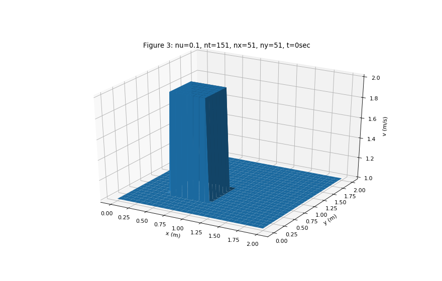
plot_3D(v,x,y,0,'Figure 3: nu=0.1, nt=151, nx=51, ny=51, t=0sec','v (m/s)')
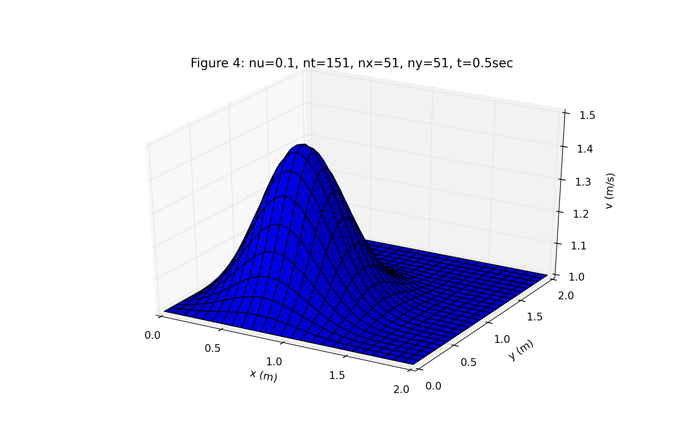
plot_3D(v,x,y,100,'Figure 4: nu=0.1, nt=151, nx=51, ny=51, t=0.5sec','v (m/s)')


7.5. Conclusions
7.5.1. Why isn’t the square wave maintained?
- As with 1D, the square wave isn’t maintained because the system is attempting to reach equilibrium - the rate of change of velocity being equal to the shear force per unit mass. There are no external forces and no convective acceleration terms.