1.1.3.1. Numerical Schemes 1
1.1.3.1.1. Setting the Scene: Stability
We encounter several instances when the solution “blows up”. Why?
Upwind schemes, implicit schemes, 2nd order schemes, leapfrog schemes
1.1.3.1.2. Consistency, stability and error analysis
Recall step one: 1D Linear Convection:
1.1.3.1.2.1. FD in time, BD in space
Explicit version:
Explicit schemes:
Very simple and economical
Restrictions for stability
Implicit version:
1.1.3.1.2.2. FD in time, CD in space
Explicit version:
Implicit version: \(n=n+1\) in the CD scheme
Results in linear system of equation with tridiagonal matrix
1.1.3.1.2.3. FD in time, FD in space
Explicit version:
Implicit version:
FD or BD in space and implicit versions are called first order upwind schemes for the convection equation.
1.1.3.1.2.4. FD in time, 2nd order BD in space
Explicit version:
Implicit version:
1.1.3.1.2.5. 2nd order CD in time, 2nd order CD in space
Explicit version: (Leapfrog scheme)
Implicit version:
1.1.3.1.3. Example
Recall step one: 1D Linear Convection:
With these initial conditions:
def diffusion(nt, nx, tmax, xmax, sigma, method):
   """
   Returns the velocity field and distance for 2D diffusion
   """
   # Increments
   dt = tmax/(nt-1)
   dx = xmax/(nx-1)

   # Compute c (given sigma)
   c = sigma * dx / dt

   # Initialise data structures
   import numpy as np
   u = np.zeros((nx,nt))
   x = np.zeros(nx)

   # X Loop
   for i in range(0,nx):
      x[i] = i*dx

   # Boundary conditions
   u[0,:] = u[nx-1,:] = 0

   # Initial conditions
   for i in range(1,nx-1):
      if(0.9<=x[i] and x[i]<=1):
         u[i,0] = 10*(x[i]-0.9)
      elif(1<x[i] and x[i]<=1.1):
         u[i,0] = 10*(1.1-x[i])
      else:
         u[i,0] = 0

   # Loop
   for n in range(0,nt-1):
      for i in range(1,nx-1):
         if(method=='BD'):
            u[i,n+1] = u[i,n]-dt*c*( ( u[i,n]-u[i-1,n] ) /dx )
         elif(method=='CD'):
            u[i,n+1] = u[i,n]-dt*c*( ( u[i+1,n]-u[i-1,n] ) / (2*dx) )

   return u, x

def plot_diffusion(u,x,nt,title):
   """
   Plots the 1D velocity field
   """
   import matplotlib.pyplot as plt
   import matplotlib.cm as cm
   plt.figure()
   colour=iter(cm.rainbow(np.linspace(0,1,nt)))
   for n in range(0,nt,1):
      c=next(colour)
      plt.plot(x,u[:,n],c=c)
      plt.xlabel('x (m)')
      plt.ylabel('u (m/s)')
      plt.title(title)
      plt.show()
u,x = diffusion(6,41, 0.2, 2.0, 0.8, 'CD')
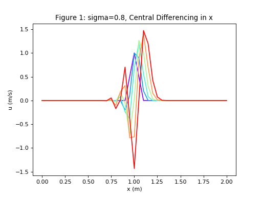
plot_diffusion(u,x,6,'Figure 1: sigma=0.8, Central Differencing in x')
u,x = diffusion(6,41, 0.2, 2.0, 0.8, 'BD')
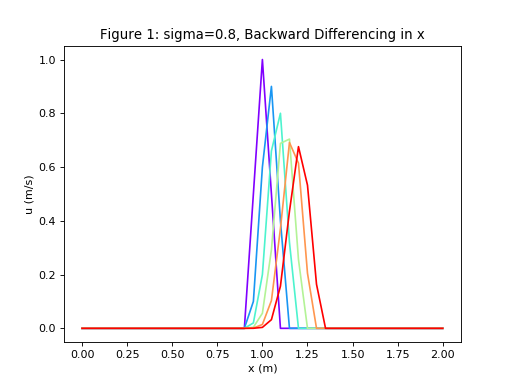
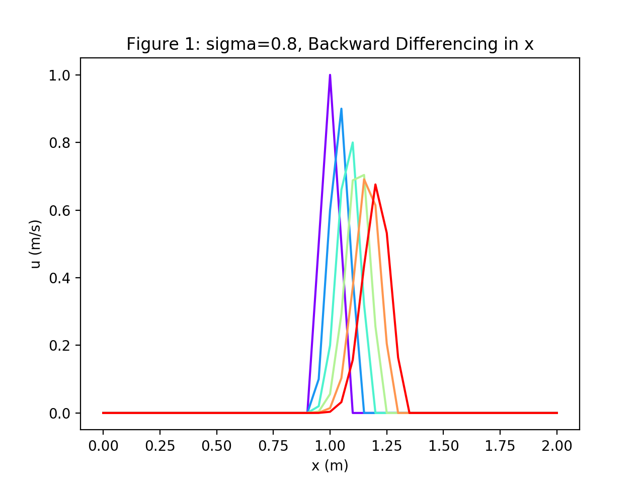
plot_diffusion(u,x,6,'Figure 1: sigma=0.8, Backward Differencing in x')
u,x = diffusion(6,41, 0.2, 2.0, 1.5, 'BD')
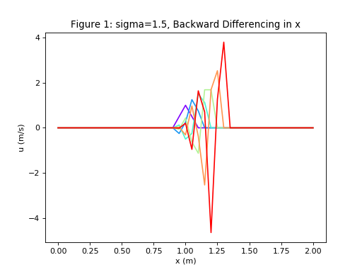
plot_diffusion(u,x,6,'Figure 1: sigma=1.5, Backward Differencing in x')

1.1.3.1.4. What Happened?
Explicit CD scheme with the parameter \(\sigma = {{c \Delta t} \over {\Delta x}} = 0.8 \Rightarrow\) UNSTABLE
1st order upwind (Step 1) BD scheme \(\sigma = 0.8 \Rightarrow\) STABLE, but significantly diffused
Do b) but with \(\sigma = 1.5 \Rightarrow\) UNSTABLE. This is conditional stability.
1.1.3.1.5. Basic Questions
What conditions should we impose on a numerical scheme to obtain an acceptable approximation to the problem?
Why do various schemes have such different behaviour?
How can we predict their stability?
For a stable scheme, how can we obtain information on the accuracy?
Need to define:
Consistency, Stability and Convergence
Truncation error - modified differential equation
Diffusion, Dispersion of the solution