1.1.10.2. The Matrix Method for Stability of Spatial Discretisation

1.1.10.2.1. The Eigenvalue Spectrum of \(\mathbf{S}\)¶

von Neumann stability analysis assumes a periodic solution and a uniform mesh

We need to establish a more general method that includes the influence of the BCs

Let \(\Omega_j\) where \(j = 1 .... N\) be eigenvalues of \(\mathbf{S}\):

\[det \left| \mathbf{S} - \Omega I \right| = 0\]

Associated eigenvectors \(V^j\) \(\Rightarrow\)

\[\mathbf{S} \cdot V^j(\mathbf{x}) = \Omega_j V^j\]

\(T\): the matrix formed by \(V^j\) as columns:

\[\mathbf{S} \cdot \mathbf{T} = \mathbf{T} \Omega\]

where:

\[\begin{split}\Omega = \begin{bmatrix} \Omega_1 & & & & \\ & \Omega_2 & & & \\ & & \ddots & & \\ & & & & \Omega_N \end{bmatrix}\end{split}\]

\[\Omega = \mathbf{T}^{-1} \mathbf{S} \mathbf{T}\]

Eigenvectors are a complete basis set

1.1.10.2.2. Recall ¶

\[{d \mathbf{u} \over dt} = \mathbf{S} \cdot \mathbf{u} + \mathbf{Q}\]

1.1.10.2.3. Model Decomposition ¶

Exact solution \(\overline{\mathbf{u}}(t,\mathbf{x})\)

\[\overline{\mathbf{u}}(t, \mathbf{x}) = \sum_{j=1}^N \overline{\mathbf{u}_j}(t) \cdot \mathbf{V}^j(\mathbf{x})\]

First term depends only on time, the second only on space.

\[Q = \sum_{j=1}^N Q_{j} V^j\]

1.1.10.2.4. Model Equation ¶

Leads to “Modal Equation” for the time dependent coefficient

\[{\overline{\mathbf{u}_j} \over t} = \Omega_j \overline{\mathbf{u}_j} + Q_j\]

The exact solution is the sum of the homogeneous solution:

\[{\overline{\mathbf{u}_{jT}} \over t} = \Omega_j \overline{\mathbf{u}_{jT}} \Rightarrow \overline{\mathbf{u}_{jT}}(t) = c_{0j} e^{\Omega_j t}\]

And a particular solution e.g. a solution of the steady state equation:

\[\Omega_j \overline{\mathbf{u}_{jS}} + Q_j = 0 \Rightarrow \overline{\mathbf{u}_{jS}} = - {Q_j \over {\Omega_j}}\]

1.1.10.2.5. Modal Solution ¶

\[\overline{\mathbf{u}_j}(t) = c_{0j} e^{\Omega_j t} - {Q_j \over {\Omega_j}}\]

Where \(c_{0j}\) are from the I.C.

IC:

\[\mathbf{u}^0(\mathbf{x}) = u(t=0, \mathbf{x})\]

In matrix representation:

\[\begin{split}\mathbf{u}^0 = \begin{bmatrix} u_0^0 \\ \vdots \\ u_i^0 \\ \vdots \\ u_{N-1} \end{bmatrix}\end{split}\]

And:

\[\mathbf{u}^0 = \sum_{j=1}^N \mathbf{u}_j^0 \mathbf{V}^j\]

At t=0 we get the coefficients

\[c_{0j} = \mathbf{u}_j^0 + {Q_j \over \Omega_j}\]

Hence:

\[\overline{\mathbf{u}_j}(t) = \mathbf{u}_j^0 e^{\Omega_j t} - {Q_j \over {\Omega_j}} \left( e^{\Omega_j t} - 1 \right)\]

The eigenvalues of the space-discretisation matrix completely determine the stability of the solution

S completely determines the behaviour of the solution!

1.1.10.2.6. Stability Condition ¶

For the ODE system:

\[{d \mathbf{u} \over dt} = \mathbf{S} \cdot \mathbf{u} + Q\]

The exact solution \(\overline{\mathbf{u}}(t,\mathbf{x})\) must remain bounded

All the modal components must be bounded

Require that exponential terms do not grow

Hence the real part of the eigenvalues must be negative or zero

(1)¶\[Re(\Omega_j) \le 0 \quad \forall j\]

\(\Omega\)- plane: The eigenvalue spectrum has to be restricted to the left half plane

Note that if (1) is satisfied:

(2)¶\[\lim_{t \Rightarrow \infty} \mathbf{u}(t) = - \sum_{j=1}^N {Q_j \over \Omega_j} V^j\]

this is a solution to the stationary problem:

\[\mathbf{S} \cdot \overline{\mathbf{u}}_S = 0\]

Want \(\Omega\) to have large negative real parts, to converge quickly to a steady state solution using an iterative method

\[exp(-Re (\Omega_j)) \Rightarrow 0\]

1.1.10.2.7. Matrix Method for Stability Analysis ¶

From the previous examples: the structure of \(\mathbf{S}\) depends on the BCs and how they are implemented (e.g. one sided difference etc)

We now have a method of investigating the influence of BCs on stability

We can also investigate effects of non-uniform meshes

More general method than von Neumann analysis

But, difficult for general boundary conditions to get analytical expressions for the eigenspectrum of \(\mathbf{S}\)

We use periodic BCs \(\Rightarrow V^j = e^{Ik_jx}\) (Fourier modes in 1D)

\[x_i = v_i^j = e^{Ik_ji \Delta x} = e^{Ii \phi_j}\]

where \(\phi_j = k_j \Delta x\)

Applied to the \(\mathbf{S}\):

\[\mathbf{S} \cdot e^{Ik_j i \Delta x} = \Omega (\phi_j)e^{Ik_j i \Delta x}\]

1.1.10.2.7.1. Example 1 - 1D Diffusion¶

CD scheme - leaving time discretisation undefined, so that we write ODEs:

\[{d u_i \over dt} = {\alpha \over \Delta x^2} (u_{i+1} - 2 u_i + u_{i-1}) = \mathbf{S} \cdot \mathbf{u}_i\]

Using eigenfunctions: \(V^j (\mathbf{x}) = e^{Ik_j x}\)

\[\mathbf{S} \cdot e^{Ik_j i \Delta x} = {\alpha \over \Delta x^2} \left( e^{Ik_j (i+1) \Delta x} - 2 e^{Ik_j i \Delta x} + e^{Ik_j (i-1) \Delta x} \right) = {\alpha \over \Delta x^2} \left( e^{Ik_j \Delta x} - 2 + e^{-Ik_j \Delta x} \right) e^{Ik_j i \Delta x} = {2 \alpha \over \Delta x^2} (cos \phi_j - 1) e^{Ik_j i \Delta x}\]

Eigenvalues are real and negative between \({-4 \alpha} / {\Delta x^2}\) and \(0\)

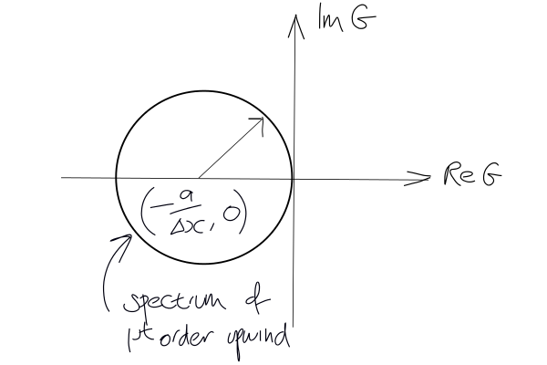
1.1.10.2.7.2. Example 2 - 1D Convection¶

With 1st order upwind

\[\left( a {du \over dx} \right) = -{a \over {\Delta x}} (u_i - u_{i-1}) = \mathbf{S} \cdot \mathbf{u}_i\]

\[\mathbf{S} \cdot e^{Ik_j i \Delta x} = -{a \over {\Delta x}} \left( e^{Ik_j i \Delta x} - e^{Ik_j (i-1) \Delta x} \right) = -{a \over {\Delta x}} \left( 1 - e^{Ik_j \Delta x} \right) e^{Ik_j i \Delta x} = -{a \over {\Delta x}} \left( 1 - cos \phi_j + I sin \phi_j \right) e^{Ik_j i \Delta x}\]

The eigenvalues are complex with negative real part, so stable

1.1.10.2.7.3. Example 3 - 1D Convection¶

With CD scheme

\[\left( a {du \over dx} \right) = -{a \over {\Delta x}} (u_{i+1} - u_{i-1}) = \mathbf{S} \cdot \mathbf{u}_i\]

\[\mathbf{S} \cdot e^{Ik_j i \Delta x} = -{a \over {\Delta x}} \left( e^{Ik_j (i+1) \Delta x} - e^{Ik_j (i-1) \Delta x} \right) = -I {a \over {\Delta x}} sin \phi_j e^{Ik_j i \Delta x}\]

The eigenvalues are imaginary in range \({{-Ia} / \Delta x}\), \({{Ia} / \Delta x}\)

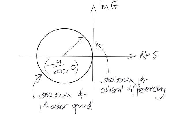
1.1.10.2.8. Conclusion ¶

All 3 examples satisfy the stability condition
Also, negative real part contributes \(e^{-\left| I Re \Omega_j \right| t }\), this creates damping
Numerical diffusion

The Visual Room