1.1.6.3. Explicit and Implicit Numerical Methods
1.1.6.3.1. Why study Non-linear Convection?
Non-linear convection is used in compressible flows
Navier-Stokes Equations are also non-linear
In incompressible flow the non-linearity usually dominates over the viscous terms
1.1.6.3.2. Inviscid Burgers Equation - Non Conservative Form
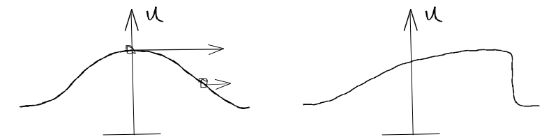
Velocity is not constant, \(u\) depends on the solution - leads to wave steepening which translates into a shock.
1.1.6.3.3. Inviscid Burgers Equation - Conservative Form
Conservative Form indicates all of the space derivatives appear in the gradient operator. Alternatively:
Physical interpretation - a wave propagating with different speeds at different points, giving rise to wave steepening, such that SHOCKS will be formed
Can use different Fluxes for different non-linear equations
Can also apply the flux to multi-dimensions, so that F becomes a vector
1.1.6.3.4. Lax-Friedrichs
1.1.6.3.4.1. Numerical Method
Explicit
1st order
1.1.6.3.4.2. Stability
Assessing stability only applies to linear equations.
Therefore, in order to study stability, we need to LINEARIZE
\(u\) is an average (or maximum) i.e. some normalising value for the speed, a local value of the solution (similar to \(c\) in the linear equation)
Consider at \(x_i\):
Recall the trigonometric functions:
From the von Neumman stability analysis and dividing by \(e^{Ii \phi}\):
For stability:
Stability now changes with the solution and depends on the solution u
1.1.6.3.5. Lax-Wendroff
1.1.6.3.5.1. Numerical Method
Consider Taylor expansion:
The equation is:
Take \(\partial / {\partial t}\)
Note that:
Where \(A\) is known as the Jacobian (used for applying the equations to higher number of dimensions)
We have:
In the case of the inviscid Burgers Equation:
Putting this into the Taylor Expansion:
Thus:
(Lax-Wendroff being a 2nd order method)
Approximate spatial derivatives with CD:
We are using a midpoint scheme for the approximation of the flux term because it allows the result to be on integer points (because the midpoint approximation is a function of integer points)
Now evaluate the Jacobian at the midpoint:
For the inviscid Burgers’ Equation \(A = u\) and \(F = {u^2 \over 2}\)
Finally we have:
1.1.6.3.5.2. Stability
Stability requires:
1.1.6.3.6. MacCormack
1.1.6.3.6.1. Numerical Method
Step 1: FTFS from \(n\) to \(n+1\) (approx)
Step 2: FTBS from \(n\) to \(n+{1 \over 2}\) with average at \(n+{1 \over 2}\):
1.1.6.3.6.2. Stability
Stability requires:
1.1.6.3.7. Beam and Warming
This is different from the explicit 2nd order upwind Beam-Warming
1.1.6.3.7.1. Taylor Expansions to replace time derivatives with spatial derivatives
Consider Taylor expansion:
Substitute (4) into (3) and absorb the O(Delta t^3) errors
Replacing the time derivatives with spatial derivatives from the Burgers’ Equation:
With an explicit scheme, the formation of the difference equation was linear (although the PDE was non-linear) by using the flux at the previous timestep (F at n)
1.1.6.3.7.2. Linearisation of Beam-Warming using the Jacobian
With an implicit scheme, we need to incorporate a linearisation system
Taylor Expansion on F:
So:
For the Burgers’ Equation:
Now take the derivative \(\partial \over \partial x\) of the previous equation:
For the second term on the RHS use 2nd order CD
Use the value of the Jacobian at the known time level \(n\) (the lagging value of the Jacobian)
1.1.6.3.7.3. Formation of the Tri-diagonal Matrix
Can now re-arrange the whole system, to form a tri-diagonal matrix.
This is a linear system of equations forming a tri-diagonal coefficient matrix
This scheme is 2nd order and unconditionally stable
There will still be oscillations, i.e. dispersion error
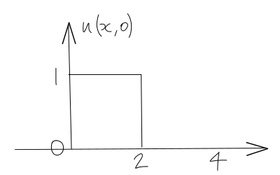
1.1.6.3.8. Practical Module - Non-linear Convection
Initial condition is a travelling shock:
Lax-Friedrichs
Lax-Wendroff
MacCormack
Beam-Warming Implicit
Beam-Warming Implicit with Damping - add on the RHS a fourth order damping term
Experiment with values of \(0 \le \epsilon_e \le 0.125\)
Try some values \(\epsilon_e \gt 0.125\)
With \(\epsilon_e = 0.1\) experiment with different step sizes and Courant numbers (\(\Delta t \over \Delta x\))
Question: Which yields the best solution for the Burgers’ Equation?
1.1.6.3.8.1. Notes on damping term
Adding a fourth order damping to a 2nd order scheme does not alter the order of accuracy of the overall method
Above, we add damping explicitly to the RHS of the equation. As a result, stability of the scheme changes, will require an upper limit in the value of the damping coefficient. Damping coefficient is require to reduce oscillations - but may not work, because the scheme may become unstable.
Typical fourth order damping (in 1D) - e means “explicit”:
Can be extended to higher dimensions
Sometimes, if 2) leads to insufficient damping. Add 2nd order implicit damping (add to LHS of the equation) - approximate with central differences
Stability analysis required to identify \((\epsilon_e)_{max}\) and also \(\epsilon_e / \epsilon_i\), typically \(\epsilon_i \gt 2 \epsilon_e\)
The damping is also called “artificial viscosity” or “artificial diffusion”