1.1.2.3. Explicit and Implicit Finite Difference Formulas¶

1.1.2.3.1. 1D Diffusion Equation¶

Recall the 1D diffusion equation (Parabolic type):

\[{\partial u \over \partial t} = \nu {\partial^2 u \over \partial x^2}\]

1.1.2.3.1.1. Explicit Solution¶

In step 3, we had:
- FD in time
- CD in space
- Equation for \(u_i^{n+1}\) was the only unknown
- Computed values at \(n+1\) depend only on past history
- To start the solution we need:
  - An Initial Condition
  - Two Boundary Conditions
- Explicit Method = a formulation of a continuum equation into a FD equation that expresses one unknown in terms of the known values

\[\left . {{u_i^{n+1} - u_i^n} \over {\Delta t}} \right \vert_{n} = \left . \nu {{u_{i+1}^{n} -2u_i^{n}+ u_{i-1}^{n}} \over \Delta x^2} \right \vert_{n}\]

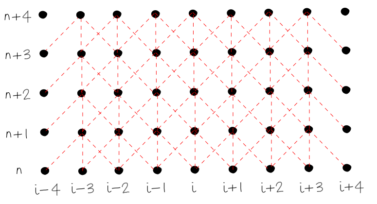
The Lag of the BCs:
- Look at the grid at time \(n+4\), the boundary conditions are imposed at \(i-4\) and \(i+4\):
- The information at the boundaries at \(n+4\) does not feed into the computations of unknowns at \(n+4\)
- This is contrary to the physics (for parabolic equations, the charactistic lines are of constant \(t\), and therefore all values at a given time level should affect the solution)
- If the BCs are constant with time, then this may not affect the solution. If the BCs vary with time, it may affect the solution
- In an explicit formula, the BCs lag behind by one step

1.1.2.3.1.2. Implicit Solution¶

How can we have a scheme that includes the BCs at every time level for the computations?
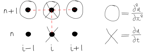
- Approximate \({\partial u} \over {\partial t}\) and \({\partial^2 u} \over {\partial x^2}\) at \(n+1\)
- So that \({\partial u} \over {\partial t}\) is effectively looking backwards in time (in other words if you took 1 off all the \(n\) values, you would get backward differencing on the LHS - but we want to march forwards on time, not backwards, so using \(n+1\) instead of \(n\) is better).

\[\left . {{u_i^{n+1} - u_i^n} \over {\Delta t}} \right \vert_{n+1} = \left . \nu {{u_{i+1}^{n+1} -2u_i^{n+1}+ u_{i-1}^{n+1}} \over \Delta x^2} \right \vert_{n+1}\]

3 unknowns, producing this stencil:

Need a set of coupled FD equations found by writing FD formulas for all grid points.

Tranpose¶

\[-r{u_{i-1}^{n+1}}+ (1+2r) {u_i^{n+1}}- r{u_{i+1}^{n+1}}=u_i^n\]

where:

\[r = \nu \left (\Delta t \over \Delta x^2 \right )\]

Linear system in matrix form will be a tri-diagonal coefficient matrix
A formulation which includes more than one unknown in the FD equation - known as an implicit method
Can use sparse methods to save memory.

Crank-Nicholson method¶

There are many numerical methods:
- Forward Differencing - 1st order, conditionally stable
- Backward Differencing - 1st order, unconditionally stable
- Crank-Nicholson - 2nd order, unconditionally stable
- Richardson - 2nd order, unconditionally unstable
- DuFort-Frankel - 2nd order, conditionally stable
Of these methods, Crank-Nicholson shows the highest accuracy and stability
Average of explicit and implicit schemes for \({\partial^2 u} \over {\partial x^2}\)
This makes \({\partial u} \over {\partial t}\) at \(n+{1 \over 2}\) represent second order central differencing in time

Numerical scheme:

\[\left . {{u_i^{n+1} - u_i^n} \over {\Delta t}} \right \vert_{n+{1 \over 2}} = \left . {1 \over 2} \nu {{u_{i+1}^{n} -2u_i^{n}+ u_{i-1}^{n}} \over \Delta x^2} \right \vert_{n} + \left . {1 \over 2} \nu {{u_{i+1}^{n+1} -2u_i^{n+1}+ u_{i-1}^{n+1}} \over \Delta x^2} \right \vert_{n+1}\]

Re-arrange in the form of the tri-diagonal matrix:

\[\left (r \over 2 \right)u_{i-1}^{n+1}+ (1+r)u_i^{n+1}- \left (r \over 2 \right)u_{i+1}^{n+1}= \left (r \over 2 \right)u_{i-1}^{n}+ (1-r)u_i^n+ \left (r \over 2 \right)u_{i+1}^{n}\]

where:

\[r = \nu {\Delta t \over \Delta x^2}\]

This is second order in time and space
Implicit \(\Rightarrow\) tridiagonal system to solve

Crank-Nicholson: Two step Interpretation¶

Note we noted before than an expression like \({u_i^{n+1}-u_i^n} \over {\Delta t}\) can be a CD approximation for the midpoint \(n+1/2\)
In terms of the grid points, we have a CD representation of \(\partial u / \partial t\) at the midpoint and the average of the diffusion at the same point
Two-step computation:

Explicit Step (FD in time, CD in space):

\[\left . {{u_i^{n+ {1 \over 2}}-u_i^n} \over {\Delta t / 2}} \right \vert_{n} = \left . \nu { {{u_{i+1}^{n} -2u_i^{n}+ u_{i-1}^{n}}} \over \Delta x^2} \right \vert_{n}\]

Implicit Step (BD in time, CD in space):

\[\left . {{u_i^{n+1}-u_i^{n+ {1 \over 2}}} \over {\Delta t / 2}} \right \vert_{n+1} = \left . \nu { {{u_{i+1}^{n+1} -2u_i^{n+1}+ u_{i-1}^{n+1}}} \over \Delta x^2} \right \vert_{n+1}\]